1.2: Evaluating Limits Analytically
In Section 1.1 we guessed limits' values by using a calculator. But these methods don't allow us to be confident in our answers. Therefore, in this section, we use limit laws to analytically evaluate limits. We discuss the following topics:
- Limit Laws
- Direct Substitution for Polynomials and Rational Functions
- Indeterminate Form \(\indZero\)
Limit Laws
We begin this discussion by introducing basic properties of limits. These laws enable us to work with constants in limits as well as limits of sums, differences, products, and quotients of functions. Remember that these rules also apply to one-sided limits.
Proving the limit laws requires the formal definition of a limit (Section 1.5), so we defer their proofs to Appendix A.2.
- \(\ds \lim_{x \to 2}[f(x) + g(x)]\)
- \(\ds \lim_{x \to 2} [f(x) - 3 g(x)]\)
- \(\ds \lim_{x \to 2} [f(x) g(x)]\)
- \(\ds \lim_{x \to 2} [5f(x)/3g(x)]\)
- The limits \(\lim_{x \to 2} f(x)\) and \(\lim_{x \to 2} g(x)\) both exist, so we use \(\eqref{eq:lim-sum}\) to obtain \[ \ba \lim_{x \to 2}[f(x) + g(x)] &= \lim_{x \to 2} f(x) + \lim_{x \to 2} g(x) \nl &= 4 + (-2) = \boxed{2} \ea \]
- We combine \(\eqref{eq:lim-diff}\) with \(\eqref{eq:lim-multiple}\) to find \[ \ba \lim_{x \to 2}[f(x) - 3 g(x)] &= \lim_{x \to 2} f(x) - \lim_{x \to 2} [3g(x)] \nl &= \lim_{x \to 2} f(x) - 3 \lim_{x \to 2} g(x) \nl &= 4 - 3 (-2) = \boxed{10} \ea \]
- Using \(\eqref{eq:lim-prod}\) gives \[ \ba \lim_{x \to 2}[f(x) g(x)] &= \lim_{x \to 2} f(x) \cdot \lim_{x \to 2} g(x) \nl &= 4 \cdot (-2) = \boxed{-8} \ea \]
- We apply \(\eqref{eq:lim-quot}\) in conjunction with \(\eqref{eq:lim-multiple},\) finding \[ \ba \lim_{x \to 2} \frac{5 f(x)}{3 g(x)} &= \frac{\ds 5 \lim_{x \to 2} f(x)}{\ds 3 \lim_{x \to 2} g(x)} \nl &= \frac{5(4)}{3(-2)} = \boxed{-\frac{10}{3}} \ea \]
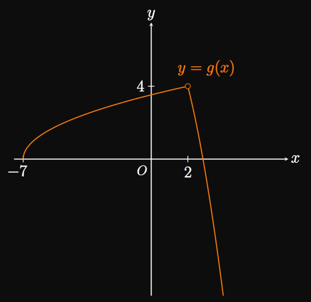
- \(\ds \lim_{x \to 0^+} [f(x)/g(x)]\)
- \(\ds \lim_{x \to -1} [2f(x) + g(x)]\)
- \(\ds \lim_{x \to \, 0 \;} [f(x) - g(x)]\)
- \(\ds \lim_{x \to \, 0 \;} [f(x) + g(x)]\)

- Inspecting the graph, we attain \[\lim_{x \to 0^+} f(x) = 4 \and \lim_{x \to 0^+} g(x) = 3 \pd \] Because the latter limit doesn't equal \(0,\) we use the Quotient Law, as in \(\eqref{eq:lim-quot},\) to find \[ \ba \lim_{x \to 0^+} \frac{f(x)}{g(x)} &= \frac{\ds \lim_{x \to 0^+} f(x)}{\ds \lim_{x \to 0^+} g(x)} \nl &= \boxed{\frac{4}{3}} \ea \]
- From the graphs, we see \[\lim_{x \to -1} f(x) = 1 \and \lim_{x \to -1} g(x) = 2 \pd \] We therefore have \[ \baat{2} \lim_{x \to -1} [2f(x) + g(x)] &= \lim_{x \to -1} [2f(x)] + \lim_{x \to -1} g(x) \comment{\text{by } \eqref{eq:lim-sum}} \nl &= 2 \lim_{x \to -1} f(x) + \lim_{x \to -1} g(x) \comment{\text{by } \eqref{eq:lim-multiple}} \nl &= 2(1) + 2 = \boxed 4 \eaat \]
- The limits \[\lim_{x \to 0} f(x) \and \lim_{x \to 0} g(x)\] both do not exist, so we cannot apply \(\eqRef{eq:lim-diff}.\) We instead consider the one-sided limits of \(\lim_{x \to 0} [f(x) - g(x)] \col\) Since \(\lim_{x \to 0^-} f(x)\) and \(\lim_{x \to 0^-} g(x)\) both exist, we can use \(\eqRef{eq:lim-diff}\) as follows: \[ \ba \lim_{x \to 0^-} [f(x) - g(x)] &= \lim_{x \to 0^-} f(x) - \lim_{x \to 0^-} g(x) \nl &= 3 - 2 = 1 \pd \nl \ea \] Likewise, the right-hand limit is \[ \ba \lim_{x \to 0^+} [f(x) - g(x)] &= \lim_{x \to 0^+} f(x) - \lim_{x \to 0^+} g(x) \nl &= 4 - 3 = 1 \pd \ea \] Since these one-sided limits are equal, we conclude \[\lim_{x \to 0} [f(x) - g(x)] = \boxed{1}\]
- Neither \(\lim_{x \to 0} f(x)\) nor \(\lim_{x \to 0} g(x)\) exists, so we can't apply \(\eqref{eq:lim-sum}\) to \(\lim_{x \to 0} [f(x) + g(x)].\) But we can apply \(\eqref{eq:lim-sum}\) to the one-sided limits: \[ \ba \lim_{x \to 0^-} [f(x) + g(x)] &= \lim_{x \to 0^-} f(x) + \lim_{x \to 0^-} g(x) = 3 + 2 = 5 \cma \nl \lim_{x \to 0^+} [f(x) + g(x)] &= \lim_{x \to 0^+} f(x) + \lim_{x \to 0^+} g(x) = 4 + 3 = 7 \pd \ea \] These values aren't equivalent, so we conclude that \(\lim_{x \to 0} [f(x) + g(x)]\) does not exist.
Limits with Powers If we use \(\eqref{eq:lim-prod}\) repeatedly with \(g(x) = f(x),\) then for any positive integer \(n\) we see \begin{align} \lim_{x \to a} \parbr{f(x)}^n &= \underbrace{\lim_{x \to a} f(x) \cdot \lim_{x \to a} f(x) \cdot \, \cdots \, \cdot \lim_{x \to a} f(x)}_{n \text{ times}} \nonum \nl &= \parbr{\lim_{x \to a} f(x)}^n \pd \label{eq:lim-power-law} \end{align} We call this property the Power Law. Now we demonstrate a special case of this law: Letting \(f(x) = x\) and using \(\eqref{eq:lim-x-a}\) show \begin{align} \lim_{x \to a} x^n &= \par{\lim_{x \to a} x}^n \nonum \nl &= a^n \pd \label{eq:lim-x^n} \end{align} The Power Law extends beyond integers; for non-integer exponents we assume \(f(x) \gt 0\) near \(a.\) Using this fact, we can take \(f(x) = x,\) replace \(n\) with \(1/n\) in \(\eqref{eq:lim-power-law},\) and use \(\eqref{eq:lim-x-a}\) to see \begin{align} \lim_{x \to a} \sqrt[n]{x} &= \lim_{x \to a} \par{x^{1/n}} \nonum \nl &= \par{\lim_{x \to a} x}^{1/n} \nonum \nl &= \sqrt[n]{\lim_{x \to a} x} \nonum \nl &= \sqrt[n]{a} \pd \label{eq:lim-sqrt-n} \end{align} (We assume \(a \gt 0\) if \(n\) is even.) More generally, it turns out that \begin{equation} \lim_{x \to a} \sqrt[n]{f(x)} = \sqrt[n]{\lim_{x \to a} f(x)} \pd \label{eq:lim-root-law} \end{equation} This formula is called the Root Law. [We assume \(\lim_{x \to a} f(x) \gt 0\) if \(n\) is even.]
Direct Substitution for Polynomials and Rational Functions
In Example 3 we see that \(f(3) = \lim_{x \to 3} f(x) = 15.\) In words, the limit of \(f(x)\) as \(x \to 3\) happens to equal \(f\) evaluated at \(3.\) This pattern is true for all polynomial and rational functions due to the Direct Substitution Property, described as follows.
As we make \(x\) arbitrarily close to \(a,\) it's intuitive that \(f\) gets closer and closer to \(f(a),\) its output at \(a.\) These well-behaved functions are called continuous; in Section 1.4 we formally discuss continuity and extend the Direct Substitution Property to all functions. Direct Substitution is very powerful—it is the main tool we use to evaluate limits analytically. Verbally, this property instructs us to evaluate \(f\) at \(a;\) the result is the value of \(\lim_{x \to a} f(x)\) if \(f\) is continuous at \(a.\) Let's prove the Direct Substitution Property for polynomial and rational functions.
PROOF
If \(f\) is an
- \(\ds \lim_{x \to 2} \par{x^2 - 5x + 7}\)
- \(\ds \lim_{x \to 1} \frac{x^3 + 3x - 2}{8x + 6}\)
- The limit is simply given by evaluating the polynomial at \(x = 2 \col\) \[ \ba \lim_{x \to 2} \par{x^2 - 5x + 7} &= (2)^2 - 5(2) + 7 \nl &= \boxed 1 \ea \]
- Replacing \(x\) with \(1\) in the rational function shows \[ \ba \lim_{x \to 1} \frac{x^3 + 3x - 2}{8x + 6} &= \frac{(1)^3 + 3(1) - 2}{8(1) + 6} \nl &= \frac{2}{14} = \boxed{\frac{1}{7}} \ea \]
Indeterminate Form \(\indZero\)
Not all rational functions can be evaluated by Direct Substitution. A limit of an indeterminate form cannot initially be evaluated by Direct Substitution because the result is inconclusive. Consider the limit \begin{equation} L = \lim_{x \to a} \frac{f(x)}{g(x)} \cmaa g(x) \ne 0 \pd \label{eq:family-of-limits} \end{equation} If both \(f(x)\) and \(g(x)\) approach \(0\) as \(x \to a,\) then \(\lim_{x \to a} [f(x)/g(x)]\) is in the indeterminate form \({\bf \indZero}.\) The numerical expression \(\indZero\) is undefined. So the quotient \(f(x)/g(x),\) where both functions approach \(0\) as \(x \to a,\) settles to an unclear number as \(x \to a\) (if the ratio even approaches a final number). A limit in an indeterminate form requires further analysis to be evaluated since it is unclear what the limit is expected to equal. But an indeterminate form does not mean the limit cannot exist. The Quotient Law doesn't apply to \(\eqref{eq:family-of-limits}\) since \(\lim_{x \to a} g(x) = 0.\) (It is also wrong to conclude that a limit doesn't exist simply because we can't apply limit laws.)
To solve limits in the indeterminate form \(\indZero,\) we use the following fact: If \(f(x) = g(x)\) when \(x \ne a,\) then \(\lim_{x \to a} f(x)\) \(= \lim_{x \to a} g(x)\) if both limits exist. The simplest method to resolve these limits is to cancel common factors. In rational functions we often encounter differences of squares, differences of cubes, and sums of cubes, which we factor as, respectively, \begin{align} a^2 - b^2 &= (a + b)(a - b) \cma \label{eq:diff-of-squares} \nl a^3 - b^3 &= (a - b)(a^2 + ab + b^2) \cma \label{eq:diff-of-cubes} \nl a^3 + b^3 &= (a + b)(a^2 - ab + b^2) \pd \label{eq:sum-of-cubes} \end{align}
Both \(\par{x^2 - 25}\) and \((x + 5)\) approach \(0\) as \(x \to -5;\) that is, Direct Substitution yields the meaningless expression \(\indZero.\) This limit is therefore of the indeterminate form \(\indZero,\) and we can't use the Quotient Law because \(\lim_{x \to -5} (x + 5) = 0.\) But since the numerator is a difference of squares, \(x^2 - 5^2,\) let's try to factor and cancel a common factor. Using \(\eqref{eq:diff-of-squares},\) we see \[ \ba \lim_{x \to -5} \frac{x^2 - 25}{x + 5} &= \lim_{x \to -5} \frac{\cancel{(x + 5)}(x - 5)}{\cancel{x + 5}} \nl &= \lim_{x \to -5} (x - 5) \nl &= \boxed{-10} \ea \]
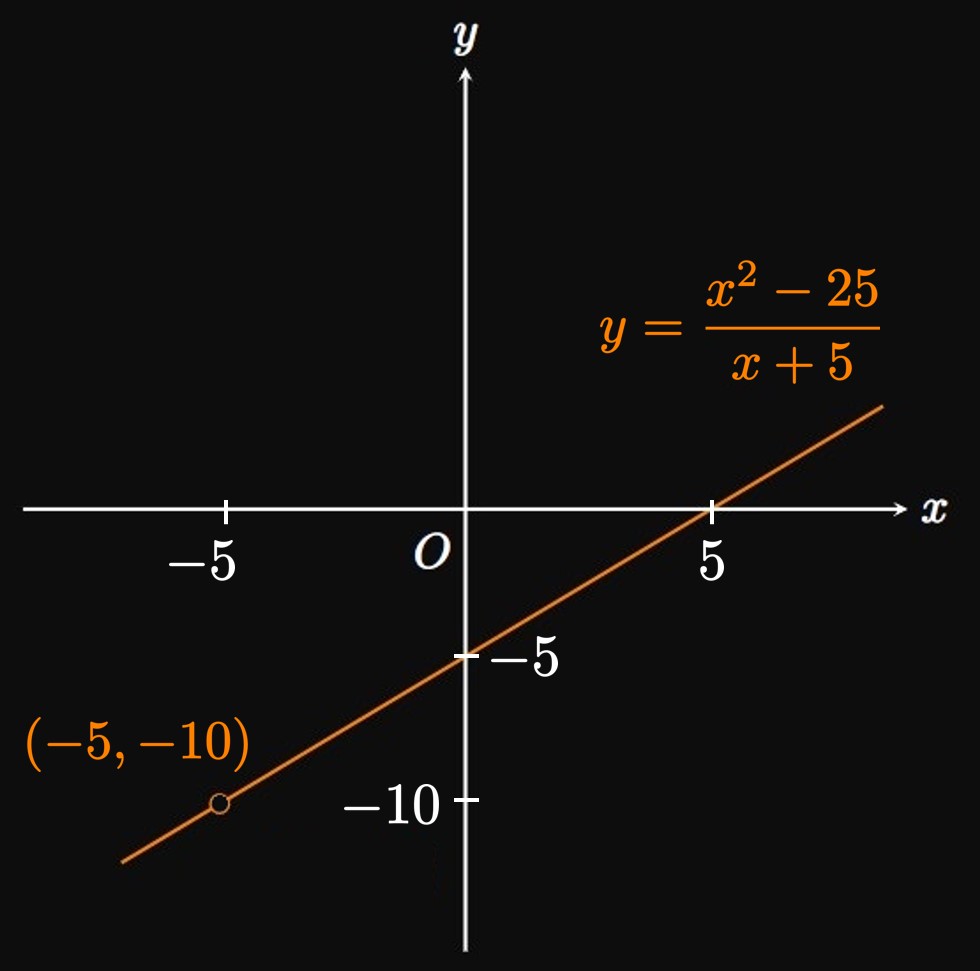
Justification The function \[f(x) = \frac{x^2 - 25}{x + 5}\] is defined for all \(x\) except \(-5,\) where its graph has a removable discontinuity (a hole), as shown in Figure 3. When we cancel the common factor \((x + 5),\) we transform \(f(x)\) into the function \(g(x) = x - 5.\) By the Direct Substitution Property, \(\lim_{x \to -5} g(x) = g(-5)\) \(= -10.\) Since \(g(x) = f(x)\) when \(x \ne -5,\) \[\lim_{x \to -5} f(x) = \lim_{x \to -5} g(x) = -10 \pd\]
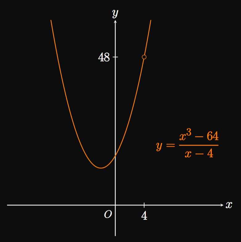
In Example 7 a limit of the indeterminate form \(\indZero\) equaled \(-10.\) But in Example 8 another limit of the indeterminate form \(\indZero\) equaled \(48.\) This contrast reveals that limits for which Direct Substitution gives \(\indZero\) can evaluate to totally different results. In fact, some limits of the indeterminate form \(\indZero\) fail to exist; others equal \(0\) or are infinite.
Rationalization In some fractions, no common factors are present in the numerator and denominator. But if either the numerator or denominator contains a radical, then we can try rationalization by multiplying across by the conjugate. [For example, the conjugate of \((4 - \sqrt x)\) is \((4 + \sqrt x);\) we simply swap the sign in the middle.] This technique is shown by the following example.
Limit Laws Limit laws enable us to calculate limits of sums, differences, products, quotients, and constants. If \(a\) and \(c\) are constants, then \begin{align} \lim_{x \to a} c &= c \cma \eqlabel{eq:lim-c} \nl \lim_{x \to a} x &= a \pd \eqlabel{eq:lim-x-a} \nl \end{align} Suppose that \(\lim_{x \to a} f(x)\) and \(\lim_{x \to a} g(x)\) both exist and that \(c\) is a constant. We then have the following properties: \begin{alignat}{2} &\lim_{x \to a} \parbr{f(x) + g(x)} = \lim_{x \to a} f(x) + \lim_{x \to a} g(x) \cma \comment{\text{Sum Law}} \eqlabel{eq:lim-sum} \nl &\lim_{x \to a} \parbr{f(x) - g(x)} = \lim_{x \to a} f(x) - \lim_{x \to a} g(x) \cma \comment{\text{Difference Law}} \eqlabel{eq:lim-diff} \nl &\lim_{x \to a} \parbr{f(x) \cdot g(x)} = \lim_{x \to a} f(x) \, \cdot \, \lim_{x \to a} g(x) \cma \comment{\text{Product Law}} \eqlabel{eq:lim-prod} \nl &\lim_{x \to a} \parbr{\frac{f(x)}{g(x)}} = \frac{\ds \lim_{x \to a} f(x)}{\ds \lim_{x \to a} g(x)} \cmaa \lim_{x \to a} g(x) \ne 0 \cma \comment{\text{Quotient Law}} \eqlabel{eq:lim-quot} \nl &\lim_{x \to a} \parbr{cf(x)} = c \lim_{x \to a} f(x) \pd \comment{\text{Constant Multiple Law}} \eqlabel{eq:lim-multiple} \end{alignat} All these properties also apply to one-sided limits. For limits with powers, let \(n\) be a positive integer; then \begin{alignat}{2} \lim_{x \to a} \parbr{f(x)}^n &= \parbr{\lim_{x \to a} f(x)}^n \cma \comment{\text{Power Law}} \eqlabel{eq:lim-power-law} \nl \lim_{x \to a} \sqrt[n]{f(x)} &= \sqrt[n]{\lim_{x \to a} f(x)} \pd \comment{\text{Root Law}} \eqlabel{eq:lim-root-law} \end{alignat} In the Root Law, we assume \(\lim_{x \to a} f(x) \gt 0\) if \(n\) is even. Special cases of these laws are as follows: \begin{align} \lim_{x \to a} x^n &= a^n \cma \eqlabel{eq:lim-x^n} \nl \lim_{x \to a} \sqrt[n]{x} &= \sqrt[n]{a} \pd \eqlabel{eq:lim-sqrt-n} \end{align} (We assume \(a \gt 0\) if \(n\) is even on the root.)
Direct Substitution for Polynomials and Rational Functions If \(f\) is a polynomial or rational function and \(a\) is in the domain of \(f,\) then \[\lim_{x \to a} f(x) = f(a) \pd\] This powerful theorem is our primary tool to evaluate many limits. Simply put, evaluate \(f\) at \(a;\) the result is \(\lim_{x \to a} f(x).\)
Indeterminate Form \(\indZero\) While Direct Substitution is powerful, not all rational functions can be initially evaluated by Direct Substitution. The limit \begin{equation} L = \lim_{x \to a} \frac{f(x)}{g(x)} \cmaa g(x) \ne 0 \eqlabel{eq:family-of-limits} \end{equation} is in the indeterminate form \(\bf \indZero\) if \(\lim_{x \to a} f(x) = 0\) and \(\lim_{x \to a} g(x) = 0.\) Limits in this form require further analysis to be evaluated. (An indeterminate form does not mean the limit cannot exist.) To resolve these limits, our primary tool is to cancel a common factor in the numerator and denominator. We use the following formulas to help expose common factors: \begin{align} a^2 - b^2 &= (a + b)(a - b) \cma \eqlabel{eq:diff-of-squares} \nl a^3 - b^3 &= (a - b)(a^2 + ab + b^2) \cma \eqlabel{eq:diff-of-cubes} \nl a^3 + b^3 &= (a + b)(a^2 - ab + b^2) \pd \eqlabel{eq:sum-of-cubes} \end{align} Alternatively, if the numerator or denominator contains a radical, then try rationalization by multiplying across by the conjugate. This process helps expose common factors to cancel.