7.1: Arc Length

So far, we have used integrals to calculate areas and volumes. The art of accumulation has enabled us to come far in our calculus journey. In this section, we extend our toolkit to calculate how long a curve is—that is, arc length. For simple shapes, we simply align a straight ruler to take measurements. But for complicated curves, this process is nearly impossible. A construction worker may want to calculate the length of a winding road. A meteorologist may wish to determine the length of a kite's trajectory. And an engineer may need to find the length of a hanging rope. These uses motivate the following topics:

• Arc Length
• Arc Length Functions

Arc Length

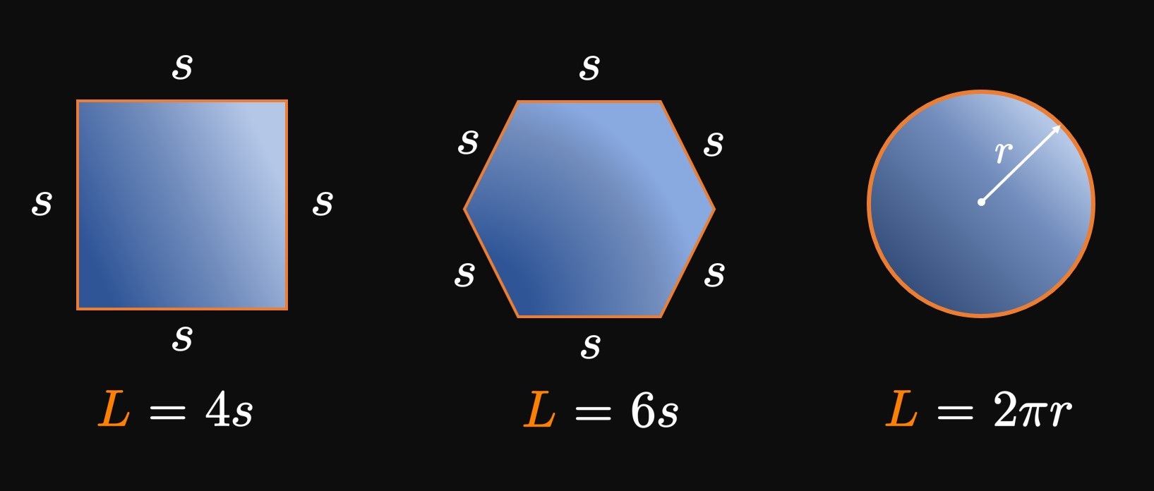
If you surround a shape with string, then the length of string you use equals the shape's perimeter. It's easy to compute the perimeter of polygons such as squares and rectangles; we sum the lengths of their sides. For example, if we wrap string around a square whose side lengths are \(s,\) then the length of string used is \(L = 4s,\) the square's perimeter. Likewise, a string of length \(L = 6s\) covers a hexagon whose sides have length \(s.\) And the circumference of a circle of radius \(r\) is \(2 \pi r,\) meaning a string of length \(L = 2 \pi r\) fully surrounds the circle. (See Figure 1.) For a curve, we call \(L\) the arc length. But how do we calculate the arc length of complicated curves?

Let \(f'\) be a continuous function on \([a, b].\) We call the corresponding graph of \(f\) smooth on \([a, b]\) because \(f'\) is continuous on this interval. To find the arc length \(L\) of \(y = f(x)\) over \(a \leq x \leq b,\) we use a polygonal approximation. Let's divide the interval \([a, b]\) into \(n\) subintervals of endpoints \(a = x_0,\) \(x_1, x_2, \dots,\) \(x_{n - 1},\) \(x_n = b\) and equal width \(\Delta x.\) In the general subinterval \([x_{i - 1}, x_i],\) the point \(P_i(x_i, y_i)\) lies on the curve \(f.\) We pivot a piece of string at the points \(P_0, P_1, \dots, P_n\) on the graph of \(f.\) (See Figure 2.) Doing so enables us to approximate \(L\) by adding the lengths of the corresponding linear line segments—namely, \begin{equation} L \approx \sum_{i = 1}^n \length{P_{i - 1} P_i} \pd \label{eq:L-approx} \end{equation} (The notation \(P_{i - 1} P_i\) is not multiplication; it denotes the line segment between points \(P_{i - 1}\) and \(P_i.\) The quantity \(\length{P_{i - 1} P_i}\) is the length of this segment.) If we increase \(n,\) then we pivot the string at more points on the curve, therefore obtaining a better approximation for \(L.\) Hence, if we let \(n \to \infty,\) then the result in \(\eqref{eq:L-approx}\) yields the exact length \(L.\) Animation 1 shows the result of increasing the number of subintervals \(n\)—the line segments better match the shape of the curve \(f.\) So we say that, if \(P_0, P_1, \dots, P_n\) are points on the graph of \(y = f(x),\) then the arc length of \(f\) over \([a, b]\) is given by \begin{equation} L = \lim_{n \to \infty} \sum_{i = 1}^n \length{P_{i - 1} P_i} \pd \label{eq:L-P} \end{equation}

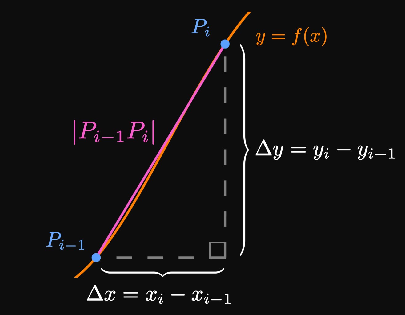
But how is \(\eqref{eq:L-P}\) useful? If we can express \(\length{P_{i - 1} P_i}\) in terms of \(x\) and \(y,\) then we attain a more applicable formula. In Figure 3, we have magnified the line segment \(P_{i - 1}P_i.\) Observe that \[\Delta x = x_i - x_{i - 1} \and \Delta y = y_i - y_{i - 1} = f(x_i) - f(x_{i - 1}) \pd\] By the Mean Value Theorem (from Section 3.2), a number \(x_i^*\) exists in \([x_{i - 1}, x_i]\) such that \[f(x_i) - f(x_{i - 1}) = f'(x_i^*) \par{x_i - x_{i - 1}} \or \Delta y = f'(x_i^*) \Delta x \pd\] Therefore, by the Pythagorean Theorem, we have \[ \ba \length{P_{i - 1} P_i} &= \sqrt{(\Delta x)^2 + (\Delta y)^2} \nl &= \sqrt{(\Delta x)^2 + \parbr{f'(x_i^*) \Delta x}^2} \nl &= \sqrt{1 + \parbr{f'(x_i^*)}^2} \sqrt{\par{\Delta x}^2} \nl &= \sqrt{1 + \parbr{f'(x_i^*)}^2} \, \Delta x \pd \ea \] Note that \(\sqrt{\par{\Delta x}^2} = \Delta x\) because \(\Delta x\) is assumed to be positive. So \(\eqref{eq:L-P}\) becomes \[ L = \lim_{n \to \infty} \sum_{i = 1}^n \sqrt{1 + \parbr{f'(x_i^*)}^2} \, \Delta x \pd \] This summation is a Riemann sum for the continuous function \(\sqrt{1 + \parbr{f'(x)}^2}\) over \(a \leq x \leq b,\) so it becomes \begin{equation} L = \int_a^b \sqrt{1 + \parbr{f'(x)}^2} \di x \pd \label{eq:L} \end{equation} If we use Leibniz notation, then we can reexpress \(\eqref{eq:L}\) as \[ L = \int_a^b \sqrt{1 + \par{\deriv{y}{x}}^2} \di x \pd \] \(\eqrefer{eq:L}\) is far more useful than \(\eqref{eq:L-P}.\) Similarly, if we integrate with \(y,\) then we attain a nearly identical formula: if \(g'\) is continuous on \([c, d],\) then the length of the smooth curve \(x = g(y)\) over \(c \leq y \leq d\) is \begin{align} L &= \int_c^d \sqrt{1 + \parbr{g'(y)}^2} \di y \label{eq:Ly} \nl &= \int_c^d \sqrt{1 + \par{\deriv{x}{y}}^2} \di y \pd \nonum \end{align}

The curve defined by the implicit equation \(y^2 = x^3\) is a semicubical parabola. Using \(\eqref{eq:L},\) calculate the length of the curve from \((0, 0)\) to \((4, 8).\) (See Figure 4.)

In Figure 5, calculate the arc length of the curve \(y = \ln(\cos x)\) from \(x = 0\) to \(x = \pi/4.\)

Figure 6 shows the portion of the parabola \(x = y^2\) from \(\par{\tfrac{1}{4}, -\tfrac{1}{2}}\) to \(\par{\tfrac{1}{4}, \tfrac{1}{2}}.\) We see \(\textderiv{x}{y} = 2y.\) Using \(\eqref{eq:Ly},\) the arc length is therefore given by \[L = \int_{-1/2}^{1/2} \sqrt{1 + (2y)^2} \di y = \int_{-1/2}^{1/2} \sqrt{1 + 4y^2} \di y \pd\] Exploiting the symmetry about the \(x\)-axis, we simplify the calculation by writing \[L = 2 \int_0^{1/2} \sqrt{1 + 4y^2} \di y \pd\] Now we perform a trigonometric substitution with \(y = \tfrac{1}{2} \tan \theta.\) (See Section 6.3 to review selecting substitutions.) Then \(\dd y = \tfrac{1}{2} \sec^2 \theta \di \theta.\) When \(y = 0,\) \(\theta = 0;\) when \(y = 1/2,\) \(\theta = \pi/4.\) So the integral becomes \[ \ba L &= 2 \int_0^{\pi/4} \sqrt{1 + \tan^2 \theta} \par{\tfrac{1}{2} \sec^2 \theta} \di \theta \nl &= \int_0^{\pi/4} \sqrt{\sec^2 \theta} \par{\sec^2 \theta} \di \theta \nl &= \int_0^{\pi/4} \abs{\sec \theta} \par{\sec^2 \theta} \di \theta \nl &= \int_0^{\pi/4} \sec^3 \theta \di \theta \pd \ea \] (The absolute value bars are dropped because secant is positive on \([0, \pi/4].\)) By Example 6.2-12, we have \[ \ba L &= \par{\tfrac{1}{2} \sec \theta \tan \theta + \tfrac{1}{2} \ln \abs{\sec \theta + \tan \theta} } \intEval_0^{\pi/4} \nl &= \parbr{\tfrac{1}{2} \par{\sqrt 2} (1) + \tfrac{1}{2} \ln \par{\sqrt 2 + 1}} - 0 \nl &= \boxed{\frac{\sqrt 2 + \ln \par{\sqrt 2 + 1}}{2}} \approx 1.148 \pd \ea \]

Arc Length Functions

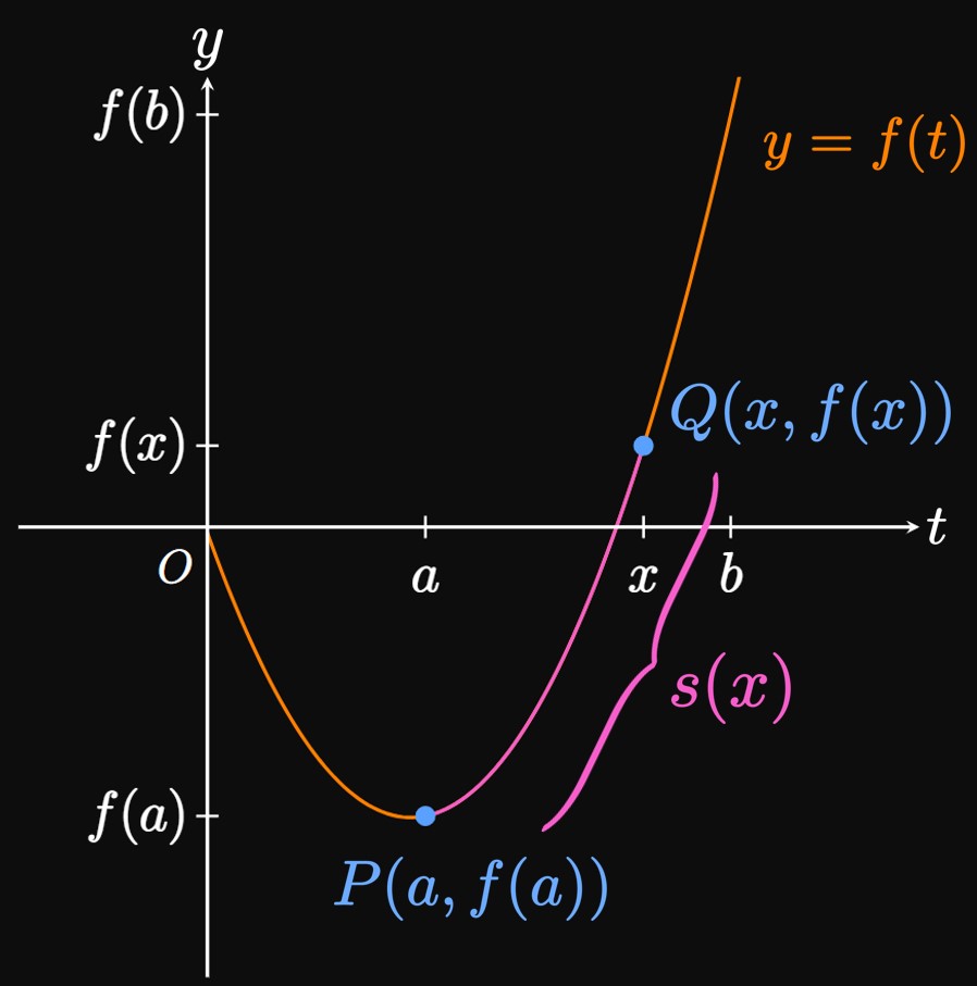
We may wish to construct an arc length function for a smooth curve. Suppose that \(f\) is smooth over \([a, b].\) Let function \(s(x)\) represent the arc length of the graph of \(y = f(t)\) from \(P(a, f(a))\) to \(Q(x, f(x)),\) where \(a \leq x \leq b.\) Using \(\eqref{eq:L},\) we therefore define \(s\) as \begin{align} s(x) &= \int_a^x \sqrt{1 + \parbr{f'(t)}^2} \di t \label{eq:s(x)} \nl &= \int_a^x \sqrt{1 + \par{\deriv{y}{t}}^2} \di t \pd \nonum \end{align} Changing the value of \(x\) shifts point \(Q,\) thus changing the arc length \(s(x)\) of \(y = f(t)\) from \(P\) to \(Q\) (Figure 7). Using Part I of the Fundamental Theorem of Calculus, we differentiate \(\eqref{eq:s(x)}\) to see \[s'(x) = \sqrt{1 + \parbr{f'(x)}^2} \cma\] which asserts that the arc length increases with the slope of the curve \(f.\) (A particle moving on the graph of \(f\) needs to travel a greater distance if the curve is steeper.) And if \(f'(x) = 0,\) then the rate at which the arc length changes with \(x\) is simply \(1.\) (Think of a particle moving along a straight line.) Thus, all arc length functions satisfy \(s'(x) \geq 1\) for \(a \leq x \leq b.\) We can also construct an arc length function with \(y\) if we interpret \(\eqref{eq:s(x)}\) in terms of quantities of \(y.\) Namely, if \(g\) is smooth on \([c, d],\) then an arc length function for the curve \(x = g(t)\) over \(c \leq y \leq d\) is given by \begin{align} s(y) &= \int_c^y \sqrt{1 + \parbr{g'(t)}^2} \di t \label{eq:s(y)} \nl &= \int_c^y \sqrt{1 + \par{\deriv{x}{t}}^2} \di t \pd \nonum \end{align}

We let \(s(x)\) be the arc length function for the curve starting at \((1, 5),\) as shown by Figure 8. Note that \(\textderiv{y}{t} = 6 \sqrt t.\) Using \(\eqref{eq:s(x)},\) we have \[s(x) = \int_1^x \sqrt{1 + \par{6 \sqrt t}^2} \di t = \int_1^x \sqrt{1 + 36 t} \di t \pd\] We substitute \(u = 1 + 36t;\) then \(\dd u = 36 \di t.\) When \(t = 1,\) \(u = 37;\) when \(t = x,\) \(u = 1 + 36x.\) So the integral becomes \[ \ba s(x) &= \tfrac{1}{36} \int_{37}^{1 + 36x} \sqrt{u} \di u \nl &= \tfrac{1}{54} \par{u^{3/2}} \intEval_{37}^{1 + 36x} \nl &= \boxed{\frac{\sqrt{(1 + 36x)^3} - 37^{3/2}}{54}} \ea \] Due to this function, we don't need to use an integral to define the arc length of \(y = 1 + 4t^{3/2}\) over \([1, x].\) For example, the arc length of the curve from \(t = 1\) to \(t = 2\) equals \[s(2) = \frac{\sqrt{[1 + 36 (2)]^3} - 37^{3/2}}{54} \approx 7.382 \pd\]