7.4: Moments and Centers of Mass
Two children can balance each other on a seesaw if they each supply equal and opposing tendencies to rotate the beam. A heavier child makes the seesaw more likely to rotate than a lighter child does; to counter this, the lighter child can sit farther from the center. On a different note, to balance a pencil on your finger, you must hold it near the center—at its center of mass. How do centers of mass relate to the degree to which a body balances and rotates? In this section we answer this question by using moments, and we learn to calculate the centers of mass of particle systems and solid plates. Then we unlock a paradoxical relationship between these ideas and volumes of solids. We discuss the following topics:
Moments and Centers of Mass for Particles
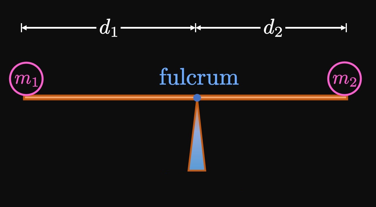
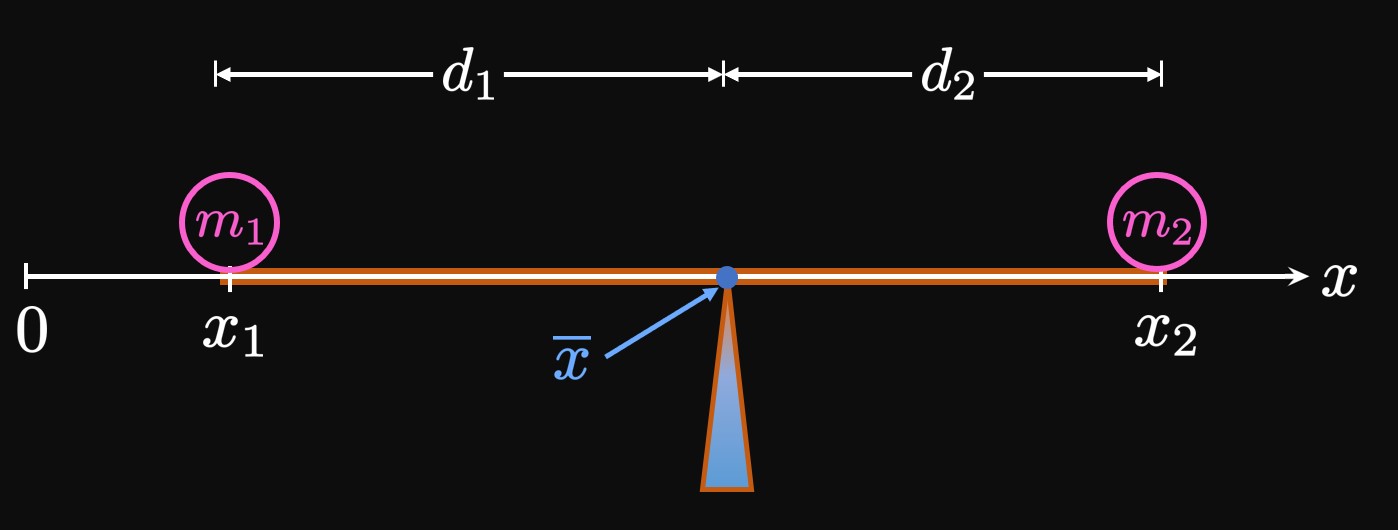
Imagine that two objects are placed on either end of a plank that pivots at some point (called the fulcrum). Let one object have mass \(m_1\) and be a distance \(d_1\) left of the fulcrum, and let the second object have mass \(m_2\) and sit a distance \(d_2\) right of the fulcrum. (See Figure 1.) The plank is balanced if \begin{equation} m_1 d_1 = m_2 d_2 \pd \label{eq:law-lever} \end{equation} (This fact is called the Law of the Lever.) Hence, a lighter object can balance a heavier object if the heavier object is placed closer to the fulcrum. Now let's use mathematics to model this balancing: Let's define a horizontal \(x\)-axis such that the \(m_1\) mass is located at \(x = x_1\) and the \(m_2\) mass is located at \(x = x_2.\) (See Figure 2.) If the fulcrum is located at \(x = \overline x,\) then we see \[d_1 = \overline x - x_1 \and d_2 = x_2 - \overline x \pd\] Substituting these expressions in \(\eqref{eq:law-lever},\) we find \begin{align} m_1 \par{\overline x - x_1} &= m_2 \par{x_2 - \overline x} \nonum \nl m_1 \overline x + m_2 \overline x &= m_1 x_1 + m_2 x_2 \nonum \nl \implies \overline x &= \frac{m_1 x_1 + m_2 x_2}{m_1 + m_2} \pd \label{eq:com-2} \end{align}
More generally, if we have \(n\) objects of masses \(m_1, m_2, \dots,\) \(m_n\) located at positions \(x_1, x_2, \dots,\) \(x_n,\) then \(\eqref{eq:com-2}\) extends to \begin{equation} \overline x = \frac{\ds \sum_{i = 1}^n m_i x_i}{\ds \sum_{i = 1}^n m_i} \pd \label{eq:com} \end{equation} This ratio gives the center of mass of a system of particles along a line—that is, the point at which the system is balanced. We call the product \(m_i x_i\) a moment; it measures the tendency for a particle to cause the system to rotate. A heavy object helps a system rotate more than a light object does, so the heavy object produces a greater moment than the light object does. Likewise, moving an object away from the center of mass increases the moment exerted because the tendency to rotate grows. In words, \(\eqref{eq:com}\) says:
The center of mass of a system of particles is given by the sum of the moments divided by the system's total mass.Therefore, a single particle of mass \(\sum_{i = 1}^n m_i\) located at \(x = \overline x\) would produce the same moment as do all \(n\) particles scattered across the \(x\)-axis.

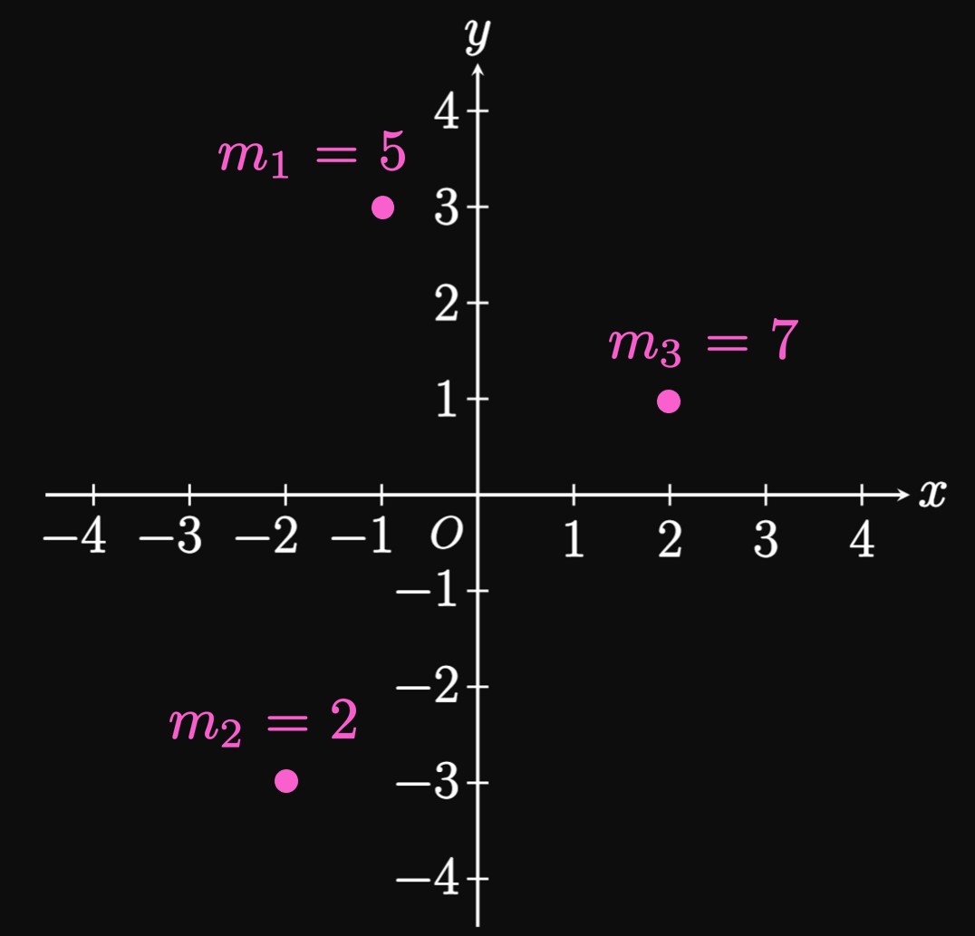
Moments in Two Dimensions In the \(xy\)-plane, consider a system of particles with masses \(m_1, m_2, \dots, m_n\) located at \(\par{x_1, y_1},\) \(\par{x_2, y_2}, \dots,\) \(\par{x_n, y_n}.\) (See Figure 3.) We define the system's moment about the \(\bf y\)-axis to be \begin{equation} M_y = \sum_{i = 1}^n m_i x_i \pd \label{eq:M-y} \end{equation} This sum measures the system's tendency to rotate about the \(y\)-axis. For the special case in Figure 1, the masses create tendencies for rotation about the vertical pivot. But placing a mass at the fulcrum causes no rotation; more generally, particles that lie on the \(y\)-axis do not help rotate the system about the \(y\)-axis. Mathematically, because \(x_i = 0,\) these particles have moments of \(0\) about the \(y\)-axis. Similarly, we define the system's moment about the \(\bf x\)-axis to be \begin{equation} M_x = \sum_{i = 1}^n m_i y_i \cma \label{eq:M-x} \end{equation} which measures the system's tendency to rotate about the \(x\)-axis. Particles that lie on the \(x\)-axis do not help rotate the system about the \(x\)-axis; since \(y_i = 0,\) their moments about the \(x\)-axis are \(0.\)
Centers of Mass in Two Dimensions Similar to the one-dimensional case, the center of mass for a system of particles in the \(xy\)-plane is given by \[ \overline x = \frac{\ds \sum_{i = 1}^n m_i x_i}{\ds \sum_{i = 1}^n m_i} \lspace \overline y = \frac{\ds \sum_{i = 1}^n m_i y_i}{\ds \sum_{i = 1}^n m_i} \pd \] Let's condense these formulas as follows: \begin{equation} \overline x = \frac{M_y}{m} \lspace \overline y = \frac{M_x}{m} \cma \label{eq:com-2d-particle} \end{equation} where \(m = \sum_{i = 1}^n m_i\) is the system's total mass.
REMARK
In Example 1,
observe that
\[
\baat{2}
\overline x &\ne -1 - 2 + 2 &&= -1 \cma \nl
\overline y &\ne 3 - 3 + 1 &&= 1 \pd
\eaat
\]
In words, the center of mass is not found by summing each mass's \(x\)- and \(y\)-coordinates.
(This would be true if the particles had equal masses.)
\(\eqReferTwo{eq:M-y}{eq:M-x}\) use the concept of weighted means;
namely, a massive particle holds a large weight
by significantly affecting the location of the center of mass.
Weighted means have other applications in probability, and they are used to compute academic grades.
Moments and Centroids of Laminae

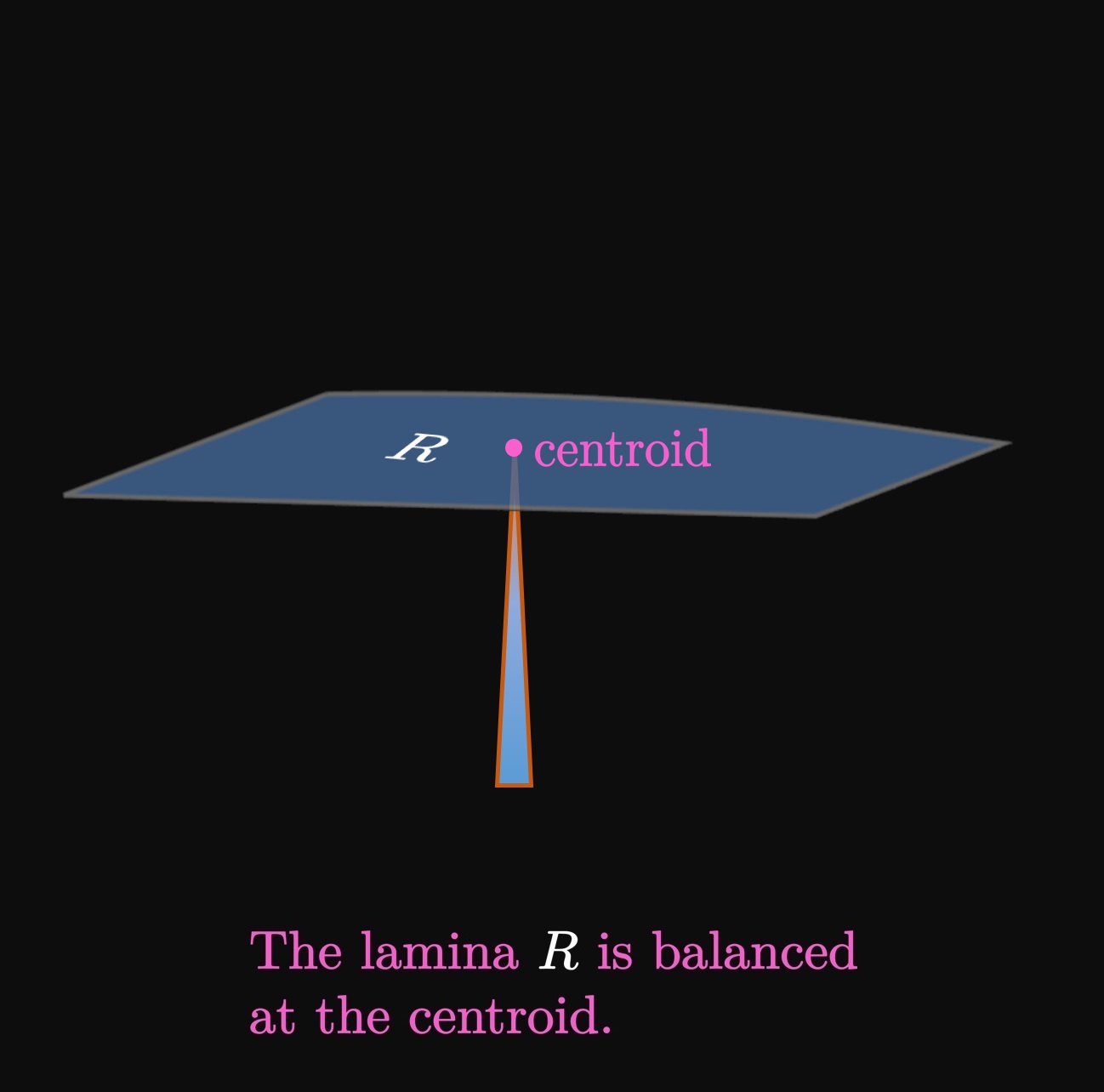
Next we focus on a flat plate of uniform surface density \(\rho;\) this body is called a lamina (plural, laminae). Its center of mass is called the centroid. In Figure 5A, a lamina's shape is the region \(R\) bounded between the curve \(y = f(x)\) and the \(x\)-axis from \(x = a\) to \(x = b;\) Figure 5B shows this lamina balanced at the centroid. Our goal is to find this lamina's centroid and its moments about the \(x\)- and \(y\)-axes. (We cannot treat this lamina as a particle.) Let's cut the lamina into \(n\) rectangles of endpoints \(a = x_0,\) \(x_1,\) \(\dots, x_{n - 1},\) \(x_n = b\) and equal width \(\Delta x,\) as in Figure 6.
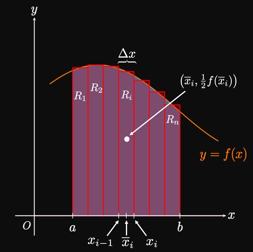
Lamina's Moment about the \(y\)-Axis We calculate each rectangle's moment about the \(y\)-axis and sum these values. In the general subinterval \(\parbr{x_{i - 1}, x_i},\) the rectangle's centroid is at its center—the point \(\par{\overline{x}_i, \tfrac{1}{2} f(\overline{x}_i)}.\) (By symmetry, the rectangle must balance at this point.) The rectangle's mass equals its density \(\rho\) multiplied by its area \(f(\overline{x}_i) \Delta x\)—namely, \[m_i = \rho f(\overline{x}_i) \Delta x \pd\] Thus, this rectangle's moment about the \(y\)-axis is equivalent to the moment about the \(y\)-axis of a particle with mass \(m_i\) placed at \(\par{\overline{x}_i, \tfrac{1}{2} f(\overline{x}_i)}.\) And this moment equals \[m_i \overline{x}_i = \rho \overline{x}_i f(\overline{x}_i) \Delta x \pd\] So if we sum the moments about the \(y\)-axis of all \(n\) rectangles, then we get \[M_y \approx \sum_{i = 1}^n \rho \overline{x}_i f(\overline{x}_i) \Delta x \pd\] This summation is a Riemann sum with the function \(\rho x f(x).\) As \(n \to \infty,\) this approximation becomes the definite integral \begin{equation} M_y = \rho \int_a^b x f(x) \di x \pd \label{eq:lamina-My} \end{equation}
Lamina's Moment about the \(x\)-Axis Similarly, let's find each rectangle's moment about the \(x\)-axis and add these numbers. Doing so estimates \(M_x,\) the lamina's moment about the \(x\)-axis. In the general subinterval \(\parbr{x_{i - 1}, x_i},\) the rectangle's centroid is a vertical distance of \(\tfrac{1}{2} f(\overline{x}_i)\) above the \(x\)-axis. With a mass of \(m_i = \rho f(\overline{x}_i) \Delta x,\) this rectangle produces a moment about the \(x\)-axis of \[m_i \par{\tfrac{1}{2} f(\overline{x}_i)} = \tfrac{1}{2} \rho [f(\overline{x}_i)]^2 \Delta x \pd\] Summing the moments about the \(x\)-axis of all \(n\) rectangles, we get \[M_x \approx \sum_{i = 1}^n \tfrac{1}{2} \rho [f(\overline{x}_i)]^2 \Delta x \pd\] As \(n \to \infty,\) we attain \begin{equation} M_x = \rho \int_a^b \tfrac{1}{2} [f(x)]^2 \di x \pd \label{eq:lamina-Mx} \end{equation}
Lamina's Centroid If the lamina's area is \(A,\) then its mass is \(m = \rho A.\) The lamina's centroid is therefore located at \[ \baat{3} \overline x &= \frac{M_y}{m} &&= \frac{\ds \rho \int_a^b x f(x) \di x}{\ds \rho A} &&= \frac{\ds \int_a^b x f(x) \di x}{\ds A} \cma \nl \overline y &= \frac{M_x}{m} &&= \frac{\ds \rho \int_a^b \tfrac{1}{2} [f(x)]^2 \di x}{\ds \rho A} &&= \frac{\ds \int_a^b \tfrac{1}{2} [f(x)]^2 \di x}{\ds A} \pd \eaat \] Observe that the \(\rho\) terms cancel. Hence, the location of a centroid is independent of the lamina's density (assuming it is constant). In summary, the region bounded by the curve \(f(x)\) and the \(x\)-axis from \(x = a\) to \(x = b\) has its centroid at \begin{equation} \overline x = \frac{1}{A} \int_a^b x f(x) \di x \lspace \overline y = \frac{1}{A} \int_a^b \tfrac{1}{2} [f(x)]^2 \di x \pd \label{eq:centroid} \end{equation}


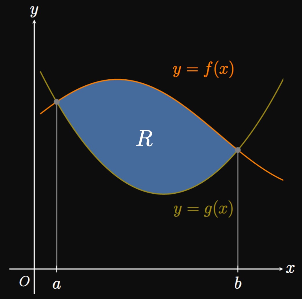
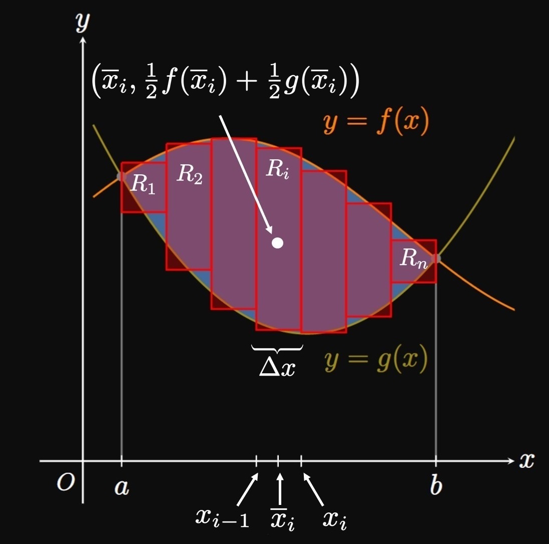
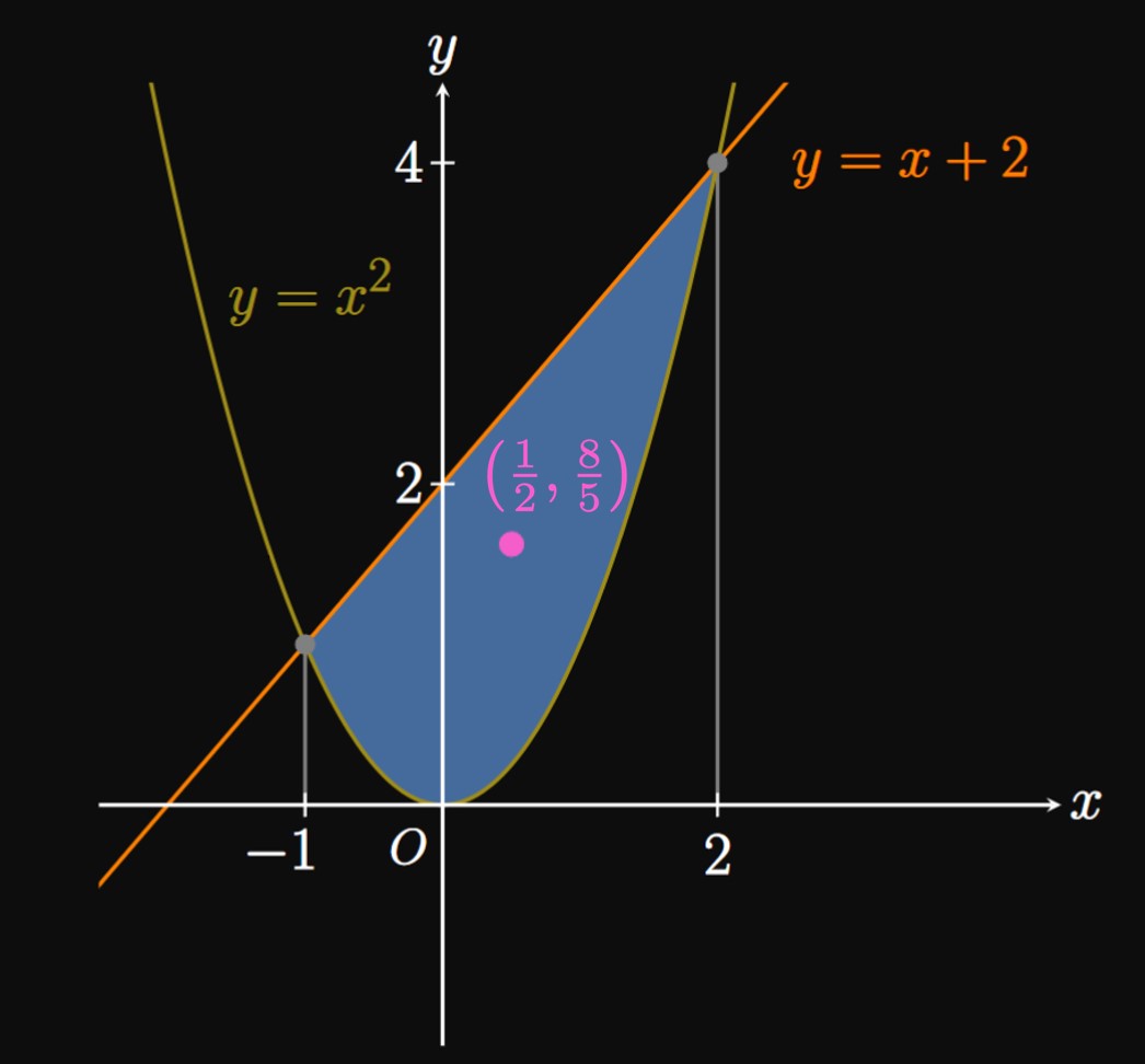
Laminae Bounded between Two Curves Suppose that a lamina of surface density \(\rho\) is bounded between the curves \(y = f(x)\) and \(y = g(x)\) from \(x = a\) to \(x = b,\) where \(f(x) \geq g(x)\) (Figure 10A). We draw \(n\) approximating rectangles, just as we did to analyze the lamina bounded by one curve. (See Figure 10B.) In the general subinterval \(\parbr{x_{i - 1}, x_i},\) the approximating rectangle's area is \([f(\overline{x}_i) - g(\overline{x}_i)] \Delta x,\) so its mass is \[m_i = \rho [f(\overline{x}_i) - g(\overline{x}_i)] \Delta x \pd\] Since the rectangle's centroid is located a distance \(\overline{x}_i\) away from the \(y\)-axis, it produces a moment about the \(y\)-axis of \[m_i \overline{x}_i = \rho \overline{x}_i [f(\overline{x}_i) - g(\overline{x}_i)] \Delta x \pd\] If we sum the moments about the \(y\)-axis of all \(n\) rectangles and take \(n \to \infty,\) then we get \begin{align} M_y &= \lim_{n \to \infty} \sum_{i = 1}^n \rho \overline{x}_i [f(\overline{x}_i) - g(\overline{x}_i)] \Delta x \nonum \nl &= \rho \int_a^b x [f(x) - g(x)] \di x \pd \label{eq:lamina-My-2} \end{align} Now observe that the approximating rectangle's centroid is above the \(x\)-axis by a distance of \[g(\overline{x}_i) + \tfrac{1}{2} [f(\overline{x}_i) - g(\overline{x}_i)] = \tfrac{1}{2} f(\overline{x}_i) + \tfrac{1}{2} g(\overline{x}_i) \pd\] Hence, this rectangle produces a moment about the \(x\)-axis of \[ \ba m_i \parbr{\tfrac{1}{2} f(\overline{x}_i) + \tfrac{1}{2} g(\overline{x}_i)} &= \rho [f(\overline{x}_i) - g(\overline{x}_i)] \parbr{\tfrac{1}{2} f(\overline{x}_i) + \tfrac{1}{2} g(\overline{x}_i)} \Delta x \nl &= \tfrac{1}{2} \rho \par{[f(\overline{x}_i)]^2 - [g(\overline{x}_i)]^2} \Delta x \pd \ea \] Summing the moments about the \(x\)-axis of all \(n\) rectangles and letting \(n \to \infty,\) we get \begin{align} M_x &= \lim_{n \to \infty} \sum_{i = 1}^n \tfrac{1}{2} \rho \par{[f(\overline{x}_i)]^2 - [g(\overline{x}_i)]^2} \Delta x \nonum \nl &= \rho \int_a^b \tfrac{1}{2} \par{[f(x)]^2 - [g(x)]^2} \di x \pd \label{eq:lamina-Mx-2} \end{align} The lamina's centroid is therefore located at \begin{equation} \overline x = \frac{1}{A} \int_a^b x [f(x) - g(x)] \di x \lspace \overline y = \frac{1}{A} \int_a^b \tfrac{1}{2} \par{[f(x)]^2 - [g(x)]^2} \di x \cma \label{eq:centroid-2} \end{equation} where \(A\) is the region's area, given by \(A = \int_a^b [f(x) - g(x)] \di x.\)
Theorem of Pappus
A surprising connection exists between centroids and solids of revolution. The Theorem of Pappus relates a region's centroid and area to the volume of the solid generated by rotating the region about an axis. This theorem, given as follows, is an alternative to the methods we developed in Chapter 5.
PROOF Let's prove the Theorem of Pappus for the case of \(\eqref{eq:pappus-y}\) in the first quadrant. By the Shell Method (from Section 5.4), the volume of the solid generated by rotating about the \(y\)-axis the region bounded between the curves \(y = f(x)\) and \(y = g(x)\) from \(x = a\) to \(x = b\) is \[V = 2 \pi \int_a^b x \parbr{f(x) - g(x)} \di x \pd\] But by \(\eqref{eq:centroid-2},\) the integral is simply \(A \overline x\) and so we attain \[V = 2 \pi \par{A \overline x} = 2 \pi A \overline x \pd\] The case of \(\eqref{eq:pappus-x}\) can be proved by swapping \(x\) and \(y\) and using a similar approach. \[\qedproof\]
- Find the centroid of \(R.\)
- Calculate the volume of the solid produced by revolving \(R\) around the \(x\)-axis.
- Calculate the volume of the solid produced by revolving \(R\) around the \(y\)-axis.
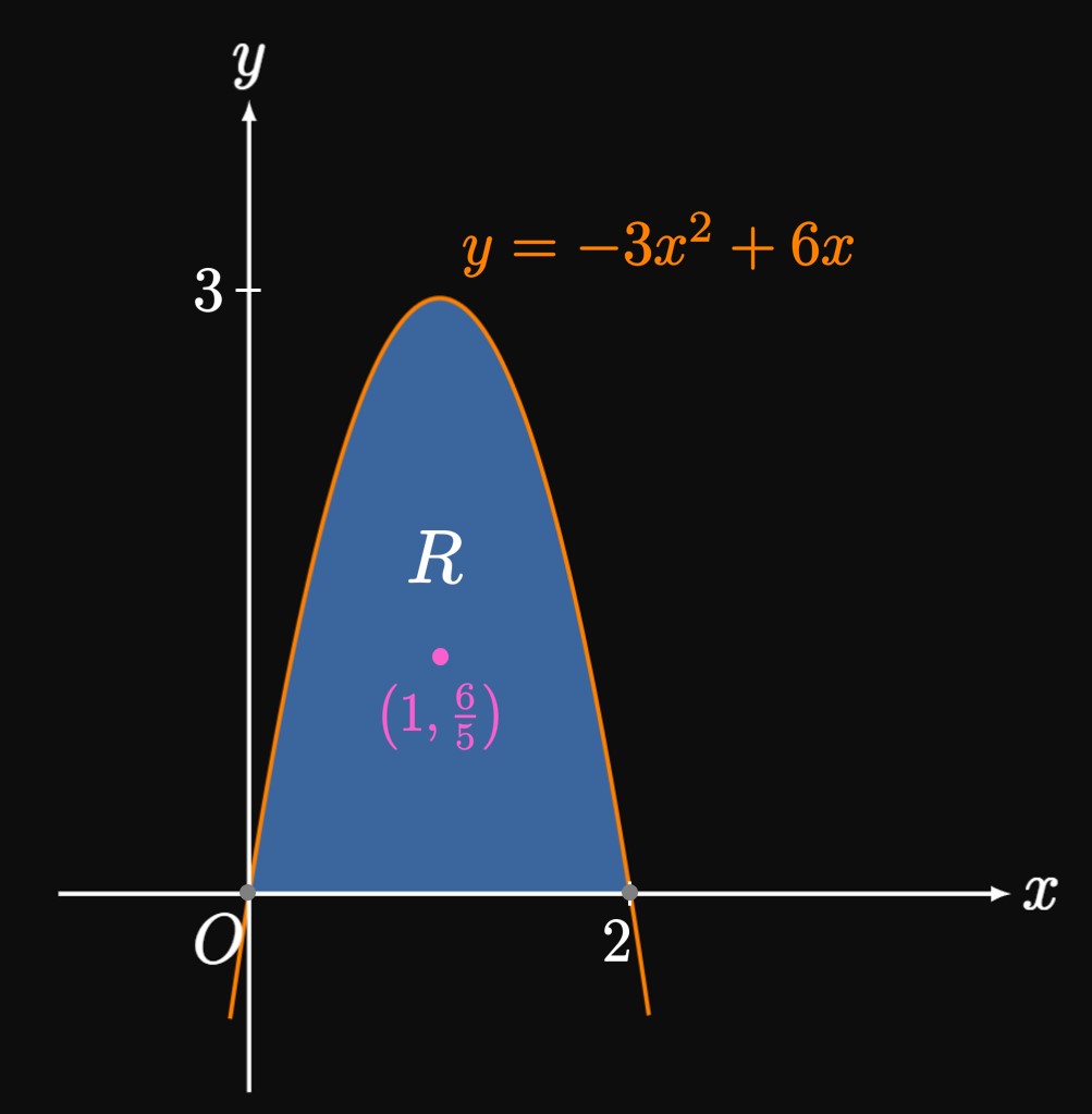
- The parabola intersects the \(x\)-axis at \(x = 0\) and \(x = 2.\) The area of \(R\) is therefore \[ \ba A &= \int_0^2 \par{-3x^2 + 6x} \di x \nl &= \par{-x^3 + 3x^2} \intEval_0^2 \nl &= 4 \pd \ea \] Because \(R\) is symmetric about \(x = 1,\) it must balance at some point on this line. We therefore argue that the \(x\)-coordinate of the centroid is \(\overline x = 1.\) By \(\eqref{eq:centroid}\) we find the \(y\)-coordinate of the centroid to be \[ \ba \overline y &= \tfrac{1}{4} \int_0^2 \tfrac{1}{2} \par{-3x^2 + 6x}^2 \di x \nl &= \tfrac{1}{8} \int_0^2 \par{9x^4 - 36x^3 + 36x^2} \di x \nl &= \tfrac{1}{8} \par{\tfrac{9}{5} x^5 - 9x^4 + 12x^3} \intEval_0^2 \nl &= \tfrac{6}{5} \pd \ea \] The centroid is therefore \(\boxed{\par{1, \tfrac{6}{5}}}\) (Figure 12).
- Using the Theorem of Pappus as in \(\eqref{eq:pappus-x},\) we find the volume to be \[ \ba V &= 2 \pi A \overline y \nl &= 2 \pi (4) \par{\tfrac{6}{5}} \nl &= \boxed{\frac{48 \pi}{5}} \approx 30.159 \pd \ea \] This method is an alternative to the Disk Method (from Section 5.3).
- By the Theorem of Pappus with \(\eqref{eq:pappus-y},\) the volume is \[ \ba V &= 2 \pi A \overline x \nl &= 2 \pi (4) (1) \nl &= \boxed{8 \pi} \approx 25.133 \pd \ea \]
Moments and Centers of Mass for Particles
A moment measures the tendency for rotation.
If \(n\) particles with masses \(m_1, m_2,\) \(\dots, m_n\)
lie along the \(x\)-axis at positions \(x_1, x_2,\) \(\dots, x_n,\)
then the
Moments and Centroids of Laminae For a thin plate (called a lamina) with uniform surface density \(\rho,\) the center of mass is given the special name of the centroid. We cannot treat this plate as a particle; we instead model it as a region bounded in the \(xy\)-plane. If a lamina of surface density \(\rho\) is the region bounded by the curve \(y = f(x)\) and the \(x\)-axis from \(x = a\) to \(x = b,\) then the moment about the \(x\)-axis is \begin{equation} M_x = \rho \int_a^b \tfrac{1}{2} [f(x)]^2 \di x \cma \eqlabel{eq:lamina-Mx} \end{equation} the moment about the \(y\)-axis is \begin{equation} M_y = \rho \int_a^b x f(x) \di x \cma \eqlabel{eq:lamina-My} \end{equation} and the centroid is located at \begin{equation} \overline x = \frac{1}{A} \int_a^b x f(x) \di x \lspace \overline y = \frac{1}{A} \int_a^b \tfrac{1}{2} [f(x)]^2 \di x \cma \eqlabel{eq:centroid} \end{equation} where \(A\) is the lamina's area. But now suppose that a lamina is bounded by two curves \(y = f(x)\) and \(y = g(x)\) from \(x = a\) to \(x = b,\) with \(f(x) \geq g(x)\) on \(a \leq x \leq b.\) Then the moment about the \(x\)-axis is \begin{equation} M_x = \rho \int_a^b \tfrac{1}{2} \par{[f(x)]^2 - [g(x)]^2} \di x \cma \eqlabel{eq:lamina-Mx-2} \end{equation} the moment about the \(y\)-axis is \begin{equation} M_y = \rho \int_a^b x [f(x) - g(x)] \di x \cma \eqlabel{eq:lamina-My-2} \end{equation} and the centroid is located at \begin{equation} \overline x = \frac{1}{A} \int_a^b x [f(x) - g(x)] \di x \lspace \overline y = \frac{1}{A} \int_a^b \tfrac{1}{2} \par{[f(x)]^2 - [g(x)]^2} \di x \pd \eqlabel{eq:centroid-2} \end{equation}
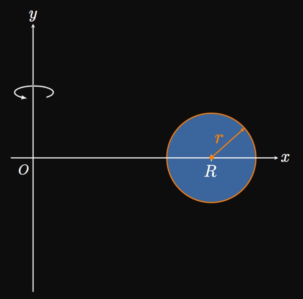
Theorem of Pappus If a region's area is \(A\) and its centroid is \(\par{\overline x, \overline y},\) and the region lies entirely on one side of the axis, then the volume of the solid generated by rotating this region about the \(x\)-axis is \begin{equation} V = 2 \pi A \abs{\overline y} \pd \eqlabel{eq:pappus-x} \end{equation} Likewise, the volume of the solid generated by rotating this region about the \(y\)-axis is \begin{equation} V = 2 \pi A \abs{\overline x} \pd \eqlabel{eq:pappus-y} \end{equation} These formulas allow us to quickly compute volumes of solids of revolution if we know a region's centroid and area.