8.3: Exponential Models

Bacteria multiplying, radioactive dating, cookies cooling—our world runs on exponential models. Exponential models are fundamental to ecology, finance, and physics. In this section, we define the mathematical basis of exponential functions and showcase a variety of applications. We discuss the following topics:

• Exponential Growth
• Compound Interest
• Exponential Decay
• First-Order Chemical Reactions
• Newton's Law of Cooling
• Discharging a Capacitor

Exponential Growth

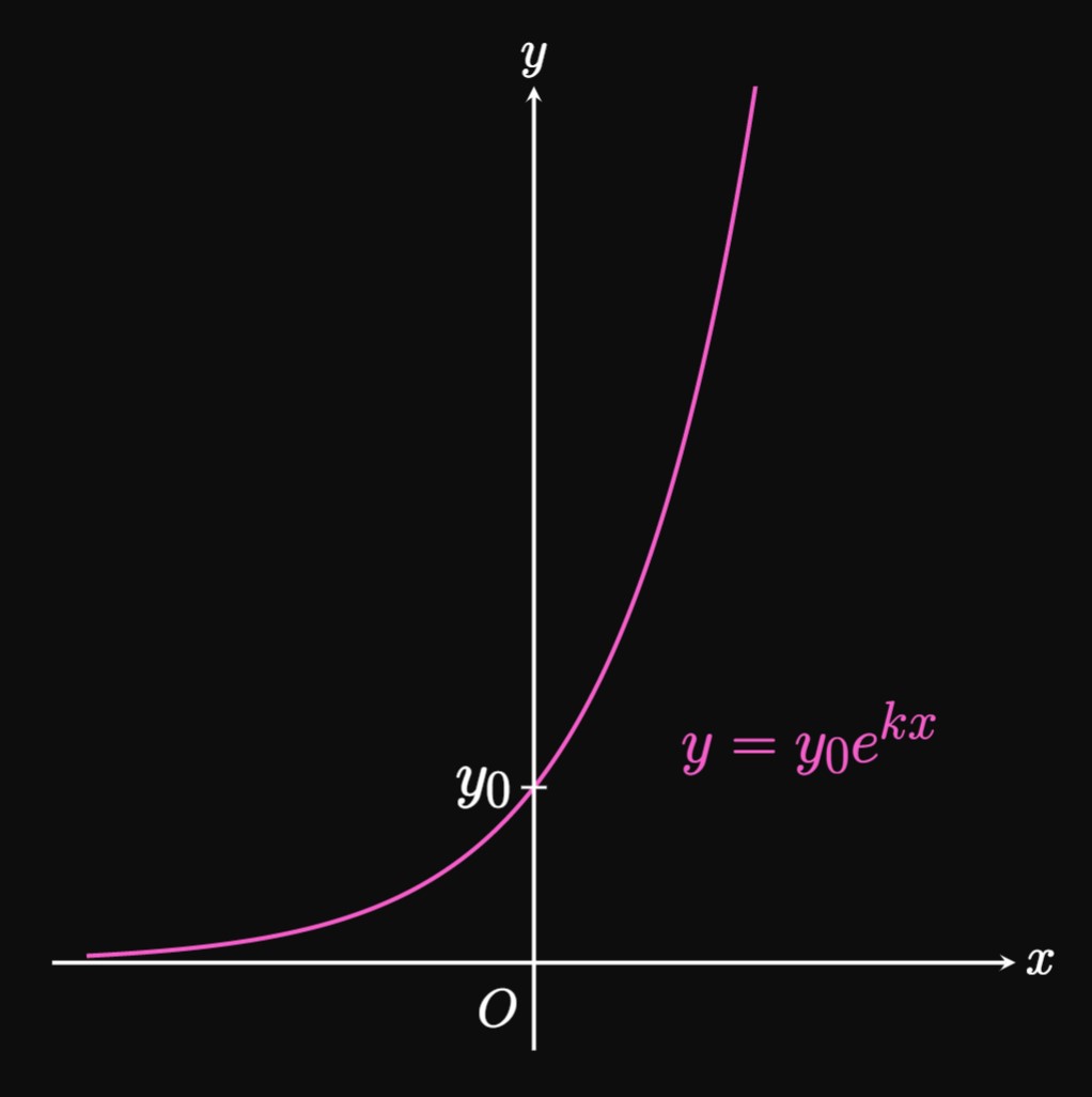
Exponential growth is a phenomenon in which a quantity undergoes very fast growth. Specifically, if \(y\) grows exponentially, then \(y\) increases at a rate proportional to itself. Mathematically, \(y\) satisfies the differential equation \begin{equation} \deriv{y}{x} = k y \comma \label{eq:exp-growth-diff-eq} \end{equation} where \(k\) is the growth constant. For clarity, we assume \(k \gt 0.\) \(\eqRefer{eq:exp-growth-diff-eq}\) asserts small values of \(y\) grow slowly and large values grow quickly. Solving for \(y\) in \(\eqref{eq:exp-growth-diff-eq}\) using Separation of Variables, we get \[ \ba \frac{1}{y} \di y &= k \di x \nl \int \frac{1}{y} \di y &= \int k \di x \nl \ln \abs{y} &= kx + C \nl y &= e^{C} e^{kx} \pd \ea \] If \(y_0\) is the value of \(y\) when \(x = 0,\) then substituting this initial condition shows \[y_0 = e^{C} e^{k(0)} = e^C \pd\] Hence, \(e^C\) is \(y_0\) and so the solution to \(\eqref{eq:exp-growth-diff-eq}\) is \begin{equation} y = y_0 e^{kx} \pd \label{eq:exp-growth} \end{equation} In Figure 1, the graph of \(y = y_0e^{kx}\) is plotted. Since its shape resembles the letter J, the curve is often called a J-curve. We obtain different graphs by changing the value of \(y_0;\) Figure 2 shows graphs of the family of graphs \(y = y_0e^{kx}\) for selected values of \(y_0.\)

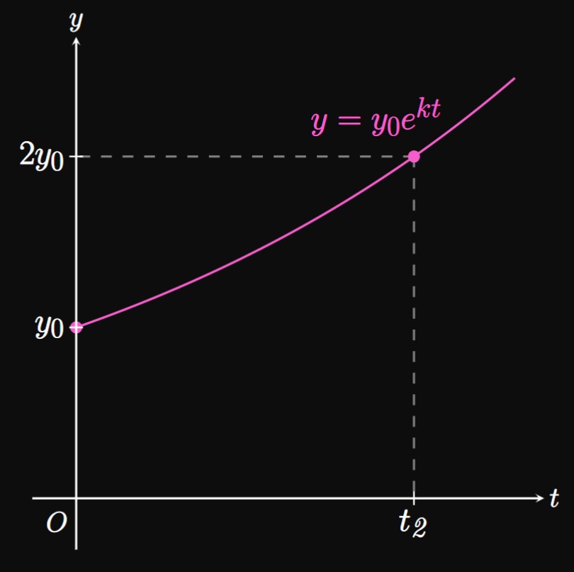
If \(y\) grows exponentially with time \(t,\) then the rate at which \(y\) grows is changing. But it turns out that \(y\) takes the same time to multiply by the same factor; for example, \(y\) takes the same time to grow from \(100\) to \(200\) as it does to grow from \(1000\) to \(2000.\) Let \(\doublingTime\) be the time that \(y\) takes to double to \(2y.\) We call \(\doublingTime\) the doubling time. Figure 3 shows the graph of \(y = y_0e^{kt},\) where \(y_0\) doubles to \(2 y_0\) after the doubling time \(\doublingTime\) has elapsed. We solve for \(\doublingTime\) by first establishing that \(y_0e^{k\doublingTime} = 2y_0.\) Then we find \begin{align} e^{k\doublingTime} &= 2 \nonumber \nl k\doublingTime &= \ln 2 \nonumber \nl \implies \doublingTime &= \frac{\ln 2}{k} \pd \label{eq:doubling-time} \end{align} In words, \(\eqrefer{eq:doubling-time}\) states that the doubling time of an exponential growth model is \(\ln 2\) divided by the growth constant.

Compound Interest

When money is lent, it earns interest. Simple interest is paid once over a time period (for example, \(1\) year). Compound interest is paid multiple times over a time period. For example, suppose that a principal amount of \(P\) dollars grows at an interest rate of \(r,\) compounded biannually (twice per year). Then after one year the amount becomes \(A = P(1 + r/2)^2,\) and after \(t\) years we have \(A = P(1 + r/2)^{2t}.\) If the interest rate is compounded three times annually at the same rate \(r,\) then the amount after \(t\) years is \(A = P(1 + r/3)^{3t}.\) This pattern continues: \[ \baat{2} A &= P \par{1 + \frac{r}{4}}^{4t} \lspace &&\text{compounded 4 times annually} \nl A &= P \par{1 + \frac{r}{5}}^{5t} \lspace &&\text{compounded 5 times annually} \nl A &= P \par{1 + \frac{r}{6}}^{6t} \lspace &&\text{compounded 6 times annually} \nl & \vdotss && \vdotss \nl \eaat \] The general pattern is, for \(r\) compounded \(n\) times annually for \(t\) time periods, \begin{equation} A = P \par{1 + \frac{r}{n}}^{nt} \pd \label{eq:compound-interest} \end{equation} But if \(r\) is continuously compounded—that is, as \(n \to \infty\)—then \(\eqref{eq:compound-interest}\) becomes \begin{equation*} A = \lim_{n \to \infty} P \par{1 + \frac{r}{n}}^{nt} \pd \end{equation*} The quantity in parentheses is the limit definition of the exponential function (see Section 2.6), so we have \begin{equation} A = Pe^{rt} \pd \label{eq:compound-interest-cont} \end{equation} We use \(\eqref{eq:compound-interest}\) if the rate \(r\) is compounded a finite number of times in a time period. This growth is discrete. In contrast, we use \(\eqref{eq:compound-interest-cont}\) for an infinite number of compounding events in a time period—that is, if a quantity grows continuously.

Exponential Decay

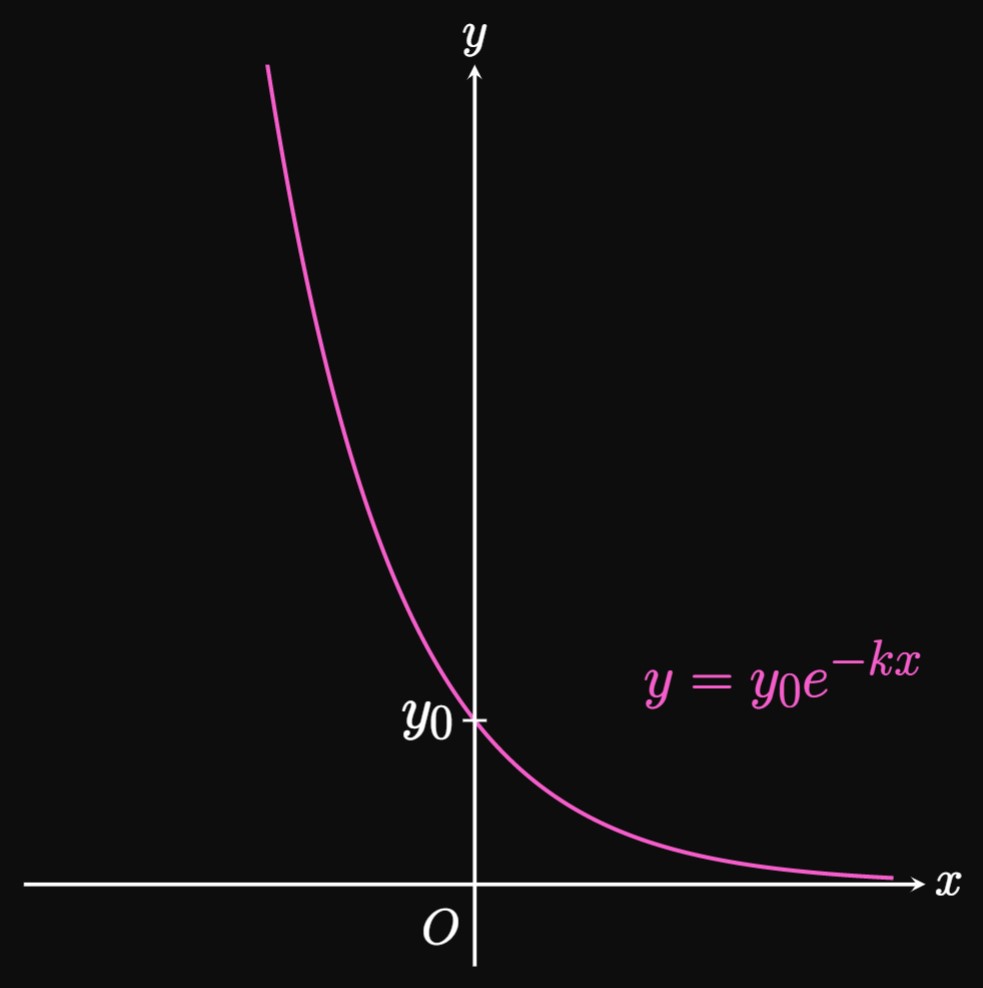
In exponential growth, the rate of increase of \(y\) is directly proportional to itself. But in exponential decay, \(y\) decreases at a rate directly proportional to itself; that is, if \(y\) decays exponentially with \(x,\) then \begin{equation} \deriv{y}{x} = -ky \pd \label{eq:exp-decay-diff-eq} \end{equation} We call \(k\) the decay constant, and we assume \(k \gt 0,\) just as we do with the growth constant. Similar to steps of obtaining \(\eqref{eq:exp-growth},\) we perform Separation of Variables for \(\eqrefer{eq:exp-decay-diff-eq} \col\) \[ \ba \frac{1}{y} \di y &= -k \di x \nl \int \frac{1}{y} \di y &= \int -k \di x \nl \ln|y| &= -kx + C \nl y &= e^{C} e^{-kx} \pd \ea \] Since \(e^C\) is the value of \(y\) when \(x = 0,\) the solution to \(\eqref{eq:exp-decay-diff-eq}\) is \begin{equation} y = y_0e^{-kx} \pd \label{eq:exp-decay} \end{equation} Whereas in exponential growth \(y\) grows very quickly, in exponential decay \(y\) decreases rapidly when \(y\) is large. Just as repeated multiplication exhibits exponential growth, repeated division shows exponential decay.

Figure 4 shows the graph of \(\eqrefer{eq:exp-decay}.\) It is a reflection of the graph of \(y = y_0e^{kx}\) (as in Figure 1) across the \(y\)-axis.

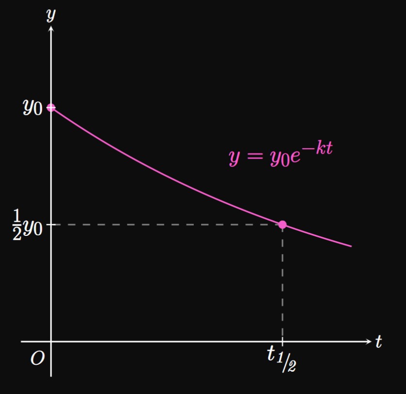
Let's suppose \(y\) decays exponentially with time \(t.\) Similar to the case of doubling time, \(y\) takes the same time to shrink by the same factor. Let \(\halfLife\) be the time \(y\) takes to reduce in half; this number is called the half-life of \(y.\) In Figure 5 the graph of \(y = y_0 e^{-kt}\) is shown, in which \(y_0\) shrinks to \(y_0/2\) at \(t = \halfLife.\) To determine an expression for \(\halfLife,\) we have \(y_0 e^{-k\halfLife} = y_0/2.\) We then have \begin{align} e^{-k \halfLife} &= \tfrac{1}{2} \nonumber \nl -k \halfLife &= \ln \tfrac{1}{2} \nonumber \nl \implies \halfLife &= \frac{\ln 2}{k} \pd \label{eq:half-life} \end{align} \(\eqrefer{eq:half-life}\) is identical to the doubling time; both expressions contain \(\ln 2\) divided by the constant \(k.\)

Knowing the half-life of a chemical compound is of value to scientists. It is a fundamental part of radioactive dating, a method of analyzing radioactive isotopes to determine the ages of rocks and minerals. Likewise, a population exposed to a dangerous material may want to know how long the substance takes to disintegrate.

First-Order Chemical Reactions

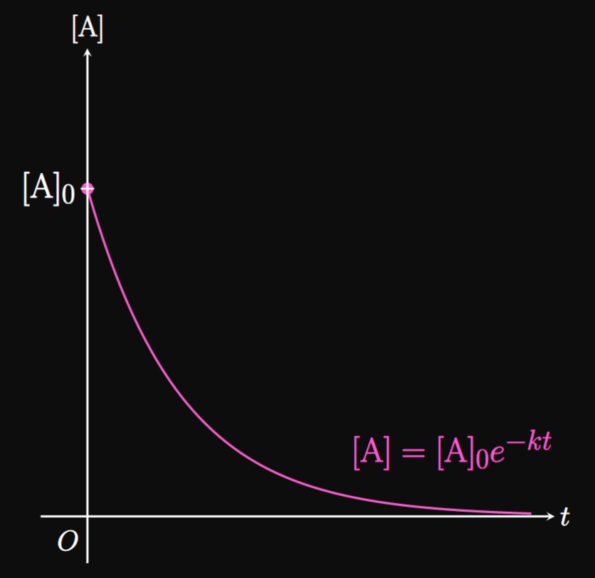
In a chemical reaction, reactants are converted into products. Let chemical substance \(\ce A\) be a reactant that forms a set of products: \begin{equation*} \ce{A -> products} \pd \end{equation*} Suppose that the rate of the reaction with time is directly proportional to the concentration of \(\ce A,\) which we write as \([\ce A].\) Then this reaction is called first-order with respect to \(\ce A.\) In other words, the rate at which \(\ce A\) is used up with time is directly proportional to the concentration of \(\ce A.\) The rate law of the reaction is a differential equation that describes the concentration of \(\ce A\)—that is, \begin{equation} \deriv{\ce{[A]}}{t} = -k \ce{[A]} \cma \label{eq:reaction-diff-eq} \end{equation} where \(k\) is called the rate constant and \(t\) is time. The integrated rate law is the solution to \(\eqref{eq:reaction-diff-eq},\) namely, \begin{equation} [\ce A] = [\ce A]_0 e^{-kt} \cma \label{eq:reaction} \end{equation} where \([\ce A]_0\) is the initial concentration of \(\ce A.\) \(\eqrefer{eq:reaction}\) asserts that when \(\ce A\) is reacted to form products, the concentration of \(\ce A\) decays exponentially with time (Figure 6).

Newton's Law of Cooling

When a hot object rests in a cool environment, Newton's Law of Cooling states that the object's temperature exhibits exponential decay with time. The temperature \(T\) decreases at a rate proportional to the difference between \(T\) and the constant surrounding temperature \(T_s.\) If \(k\) is the decay constant and \(t\) is time, then the law gives the differential equation \begin{equation} \deriv{T}{t} = -k(T - T_s) \pd \label{eq:newtons-cooling-diff-eq} \end{equation}

The graph of \(\eqrefer{eq:newtons-cooling}\) is illustrated in Figure 7: The object's temperature \(T\) begins at \(T_0\) before leveling off to \(T_s,\) the surrounding temperature. Note that \(T\) is always above \(T_s,\) which is logical because the cooling object shouldn't reach a temperature below the ambient temperature. This model assumes that the object's heat dissipation does not warm up the surrounding environment. If the object is small—for example, a cup of hot tea or a freshly baked cookie—then this assumption is appropriate.

Discharging a Capacitor

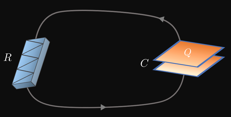
A resistance–capacitance (RC) circuit consists of a capacitor and resistor. A capacitor is a device that stores electrical energy on one of its conducting surfaces, and capacitance \(C\) (unit, farads) is the ability of a capacitor to hold a charge \(Q\) (unit, coulombs). In Figure 8, a charged capacitor is connected to a resistor of resistance \(R\) (unit, ohms). As current travels through the circuit, the capacitor is discharging and the resistance dissipates the energy in the circuit. Applying Kirchhoff's Loop Rule gives the differential equation \[\frac{Q}{C} + R \deriv{Q}{t} = 0 \pd\] Solving for \(\textDeriv{Q}{t}\) and letting \(\tau = RC\) (\(\tau\) is the greek letter tau), we attain \begin{equation} \deriv{Q}{t} = -\frac{1}{\tau} Q \pd \label{eq:rc-diff-eq} \end{equation} We compare \(\eqref{eq:rc-diff-eq}\) \([\textDeriv{Q}{t} = -(1/\tau)Q]\) to \(\eqref{eq:exp-decay-diff-eq}\) \([\textDeriv{y}{x} = -ky]\) by identifying \(k = 1/\tau.\) Through this comparison, we see that large values of \(\tau\)—called the time constant of an RC circuit—cause \(Q\) to decay slowly because the decay constant \(1/\tau\) is small. In contrast, small values of \(\tau\) enable \(Q\) to dissipate quickly due to the large decay constant. This interpretation is logical, since resistance \(R\) impedes the flow of current and capacitance \(C\) allows the capacitor to store charge; so large values of either quantity slow the capacitor's discharge. If \(Q_0\) is the initial charge on the capacitor, then the solution to \(\eqref{eq:rc-diff-eq}\) is \begin{equation} Q = Q_0 e^{-t/\tau} \pd \label{eq:rc-Q} \end{equation}

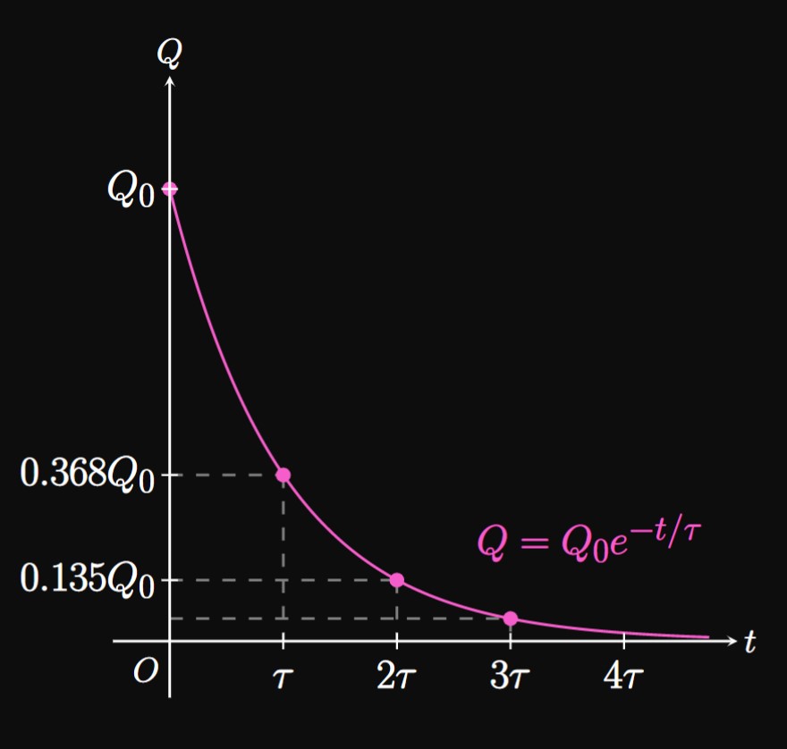
Similar to how half-lives are a standard to measure decay, the level of charge \(Q\) on the capacitor can be gauged by how many time constants have elapsed. If \(t = \tau,\) then \(\eqref{eq:rc-Q}\) becomes \(Q = Q_0 e^{-1} \approx 0.368 Q_0.\) Likewise, if \(t = 2 \tau\) then \(\eqref{eq:rc-Q}\) gives \(Q = Q_0 e^{-2} \approx 0.135Q_0.\) Thus, after one time constant has elapsed, approximately \(63.2 \%\) of the capacitor's charge has been dissipated. After two time constants have passed, approximately \(86.5\%\) of the charge has been lost. This pattern is represented by the graph in Figure 9.