Chapter 8 Challenge Problems Solutions
- Show that \(f'(x) = k f(x)\) for all \(x.\)
- Determine the identity of \(f.\)
- The property \(f(a + b) = f(a) f(b)\) is called the Multiplicative Cauchy functional equation. By interpreting your result from part (b), what is the only family of elementary, real-valued, non-constant functions on \(\RR\) that satisfy this relation?
- Taking \(a = x\) and \(b = h\) shows \[f(x + h) = f(x) f(h) \pd\] By the limit definition of a derivative (Section 2.1), \[ \ba f'(x) &= \lim_{h \to 0} \frac{f(x + h) - f(x)}{h} \nl &= \lim_{h \to 0} \frac{f(x) f(h) - f(x)}{h} \nl &= f(x) \lim_{h \to 0} \frac{f(h) - 1}{h} \pd \ea \] Since \(f(0) = 1,\) note that \[\lim_{h \to 0} \frac{f(0 + h) - f(0)}{h} = f'(0) \pd\] (Alternatively, you could use L'Hôpital's Rule to resolve the limit.) But \(f'(0) = k,\) so we have \[f'(x) = k f(x) \cma\] as requested.
- The differential equation \(f'(x) = k f(x)\) can be rewritten as \[ \deriv{y}{x} = k y \cma \] where \(y = f(x).\) Using Separation of Variables, we see \[ \ba \int \frac{\dd y}{y} &= \int k \di x \nl \ln \abs y &= kx + C_1 \nl \abs y &= e^{C_1} e^{kx} \nl y &= C e^{kx} \cma \ea \] where \(C = \pm e^{C_1}.\) Substituting \(y(0) = 1\) shows \[1 = C e^{0} \implies C = 1 \pd\] Thus, the identity of \(f\) is \[f(x) = \boxed{e^{kx}}\]
- Exponential functions in the form \(f(x) = e^{kx},\) \(k \ne 0,\) satisfy the Multiplicative Cauchy functional equation.
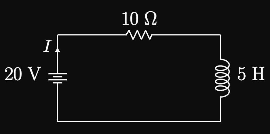
- Using Euler's Method with step size \(h = 0.25,\) approximate the current after \(1\) second has elapsed.
-
What is the current after a very long time (that is, as
\(t \to \infty\))? - The particular solution to the differential equation turns out to be \[I(t) = 2 \par{1 - e^{-2t}} \pd\] Verify this result. Does this function make physical sense?
- We have the initial condition \(I(0) = 0.\) Let's rewrite the given differential equation as \[\deriv{I}{t} = 4 - 2I \pd\] The first step of Euler's Method gives \[I_1 = 0 + 0.25 \parbr{4 - 2(0)} = 1 \un A \pd\] Likewise, subsequent approximations are as follows: \[ \ba I_2 &= 1 + 0.25 \parbr{4 - 2(1)} = 1.5 \un A \cma \nl I_3 &= 1.5 + 0.25 \parbr{4 - 2(1.5)} = 1.75 \un A \cma \nl I(1) \approx I_4 &= 1.75 + 0.25 \parbr{4 - 2(1.75)} = \boxed{1.875 \un A} \ea \]
- We see \(\textderiv{I}{t} \to 0\) as \(I \to 2,\) meaning \(I\) cannot increase past \(2 \un A.\) Thus, the current after a very long time is \(\boxed{2 \un A}.\)
- Differentiating \(I,\) we attain \[I'(t) = 4e^{-2t} \pd\] We then see \[20 - \underbrace{10 \parbr{2\par{1 - e^{-2t}}}}_{10 I} - \underbrace{5 \par{4e^{-2t}}}_{5 \, \textderiv{I}{t}} \equalsCheck 0 \pd\] In addition, the initial condition \(I(0) = 0\) is met: \[I(0) = 2 \par{1 - e^0} \equalsCheck 0 \pd\] Hence, \(I(t) = 2 \par{1 - e^{-2t}}\) is a particular solution because it satisfies the differential equation with \(I(0) = 0.\) The solution makes physical sense because the inductor gradually allows more current to flow in the circuit. Initially, the inductor opposes most of the current from flowing, but it eventually allows the current to grow to its maximum of \(2 \un A.\) With this behavior, inductors are used as shut-off devices—for example, in surge protectors—to prevent electronic damage by a current overload.
Velocity Function Recall that acceleration is the time derivative of velocity—that is, \(a = \textderiv{v}{t}.\) Given \(a^2 = 1 - 4v^2,\) we have the following differential equation: \[ \deriv{v}{t} = \pm \sqrt{1 - 4v^2} \pd \] Because \(v(0) = 1/2\) ensures the right side equals \(0,\) \(\textderiv{v}{t} = \pm \sqrt{1 - 4v^2}\) agree at \(t = 0.\) It turns out that choosing either branch yields the same volution, as we will see later. Performing Separation of Variables gives \[\int \frac{1}{\sqrt{1 - 4v^2}} \di v = \int \dd t \pd\] To evaluate the integral on the left, we substitute \(u = 2v.\) Then \(\dd u = 2 \di v\) and so \[ \ba \int \frac{1}{\sqrt{1 - 4v^2}} \di v &= \int \frac{1/2}{\sqrt{1 - u^2}} \di u \nl &= \tfrac{1}{2} \asin u \nl &= \tfrac{1}{2} \asin 2v \cma \ea \] where we omitted the constant of integration. We therefore have \[\tfrac{1}{2} \asin 2v = t + C \pd\] Substituting the initial condition \(v(0) = 1/2,\) we find \[\tfrac{1}{2} \asin 1 = 0 + C \implies C = \frac{\pi}{4} \pd\] Hence, we have \[ \ba \tfrac{1}{2} \asin 2v &= t + \frac{\pi}{4} \nl \asin 2v &= 2t + \frac{\pi}{2} \nl 2v &= \sin \par{2t + \frac{\pi}{2}} \nl v(t) &= \boxed{\tfrac{1}{2} \sin \par{2t + \frac{\pi}{2}}} \ea \] Note that \(v(t)\) is even. If the negative branch of the square root were selected in the differential equation, then the solution would be \[v(t) = \tfrac{1}{2} \sin \par{-2t + \frac{\pi}{2}} \cma\] which is equivalent to our answer.
Acceleration Function The acceleration function is given by \(a(t) = \textderiv{v}{t},\) namely, \[ \ba a(t) &= \deriv{}{t} \parbr{\tfrac{1}{2} \sin \par{2t + \frac{\pi}{2}}} \nl &= \boxed{\cos \par{2t + \frac{\pi}{2}}} \ea \]
Position Function The position function is given by \(s(t) = \int v(t) \di t,\) that is, \[s(t) = \int \tfrac{1}{2} \sin \par{2t + \frac{\pi}{2}} \di t \pd\] Substituting \(u = 2t + \pi/2,\) we have \(\dd u = 2 \di t\) and therefore \[ \ba \int \tfrac{1}{2} \sin \par{2t + \frac{\pi}{2}} \di t &= \int \tfrac{1}{4} \sin u \di u \nl &= - \tfrac{1}{4} \cos u + D \nl &= -\tfrac{1}{4} \cos \par{2t + \frac{\pi}{2}} + D \pd \ea \] Accordingly, the position function is \[s(t) = -\tfrac{1}{4} \cos \par{2t + \frac{\pi}{2}} + D \pd\] Since \(s(0) = 0,\) we find \[0 = -\tfrac{1}{4} \cos \par{0 + \frac{\pi}{2}} + D \implies D = 0 \pd\] Thus, the position function is \[s(t) = \boxed{-\tfrac{1}{4} \cos \par{2t + \frac{\pi}{2}}}\]
- It can be shown that the transient solution to the differential equation takes the form \[x_T(t) = C e^{-\lambda t} \cos \par{\alpha t + \beta} \cma\] where \(C,\) \(\lambda,\) \(\alpha,\) and \(\beta\) are nonzero constants with \(\lambda \gt 0.\) Show that \(x_T(t) \to 0\) as \(t \to \infty.\) What does this result mean?
- The steady-state solution can be assumed to be of the form \[x_S(t) = A \cos \omega t + B \sin \omega t \pd\] Substitute this function into the differential equation to solve for \(A\) and \(B.\) (Hint: Compare the coefficients of the sine and cosine terms.)
- The amplitude of the object's displacement is \(X = \sqrt{A^2 + B^2}.\) Using the result of part (b), find \(X.\)
-
We aim to show that
\[\lim_{t \to \infty} x_T(t) = \lim_{t \to \infty} C e^{-\lambda t} \cos \par{\alpha t + \beta} = 0 \pd\]
Because cosine's range is \([-1, 1],\) we have \(-1 \leq \cos \par{\alpha t + \beta} \leq 1.\)
In addition, \(-\abs C \leq C \leq \abs C,\) so
\[-\abs C e^{-\lambda t} \leq C e^{-\lambda t} \cos \par{\alpha t + \beta} \leq \abs C e^{-\lambda t} \pd\]
Since \(\lambda \gt 0,\) we see
\[\lim_{t \to \infty} \par{-\abs C e^{-\lambda t}} = \lim_{t \to \infty} \par{\abs C e^{-\lambda t}} = 0 \pd\]
Hence, by the Squeeze Theorem, \(\lim_{t \to \infty} x_T(t) = 0.\)
Accordingly, the transient solution
dies out
over time, and the system's behavior is governed by \(x_S(t)\) as \(t \to \infty.\) - Differentiating \(x_S(t) = A \cos \omega t + B \sin \omega t\) shows \[ \ba \deriv{x_S}{t} &= -A \omega \sin \omega t + B \omega \cos \omega t \cma \nl \derivOrder{x_S}{t}{2} &= -A \omega^2 \cos \omega t - B \omega^2 \sin \omega t \pd \ea \] Substituting these expressions into the differential equation yields \[ \small \ba m \par{-A \omega^2 \cos \omega t - B \omega^2 \sin \omega t} + c \par{-A \omega \sin \omega t + B \omega \cos \omega t} + k \par{A \cos \omega t + B \sin \omega t} &= F_0 \cos \omega t \nl \par{-mA \omega^2 + Bc \, \omega + kA} \cos \omega t + \par{-m B \omega^2 - A c \, \omega + kB} \sin \omega t &= F_0 \cos \omega t \pd \ea \] On both sides, the coefficients of the cosines must match, so \begin{equation} -mA \omega^2 + Bc \, \omega + kA = F_0 \pd \label{eq:response-cos} \end{equation} In addition, the coefficients of the sines must match, meaning \begin{equation} -m B \omega^2 - A c \, \omega + kB = 0 \pd \label{eq:response-sin} \end{equation} From \(\eqref{eq:response-sin},\) solving for \(B\) gives \[B = A \, \frac{c \, \omega}{k - m \omega^2} \pd\] Substituting this result into \(\eqref{eq:response-cos}\) shows \[ \ba A \par{k - m \omega^2} + \par{A \, \frac{c \, \omega}{k - m \omega^2}} (c \, \omega) &= F_0 \nl \implies A &= \frac{F_0}{k - m \omega^2 + \frac{(c \, \omega)^2}{k - m \omega^2}} \nl &= \boxed{\frac{F_0 \par{k - m \omega^2}}{\par{k - m \omega^2}^2 + \par{c \, \omega}^2}} \ea \] Then \[B = \boxed{\frac{F_0 (c \, \omega)}{\par{k - m \omega^2}^2 + (c \, \omega)^2}}\] The steady-state solution is therefore \[x_S(t) = \frac{F_0 \par{k - m \omega^2}}{\par{k - m \omega^2}^2 + \par{c \, \omega}^2} \cos \omega t + \frac{F_0 c \, \omega}{\par{k - m \omega^2}^2 + (c \, \omega)^2} \sin \omega t \pd \]
- We have \[ \ba X &= \sqrt{A^2 + B^2} \nl &= \sqrt{\par{\frac{F_0 \par{k - m \omega^2}}{\par{k - m \omega^2}^2 + \par{c \, \omega}^2}}^2 + \par{\frac{F_0 (c \, \omega)}{\par{k - m \omega^2}^2 + (c \, \omega)^2}}^2} \nl &= \sqrt{\frac{\par{F_0}^2 \parbr{\par{k - m \omega^2}^2 + (c \, \omega)^2}}{\parbr{\par{k - m \omega^2}^2 + \par{c \, \omega}^2}^2}} \nl &= \sqrt{\frac{\par{F_0}^2}{\par{k - m \omega^2}^2 + \par{c \, \omega}^2}} \nl &= \boxed{\frac{F_0}{\sqrt{\par{k - m \omega^2}^2 + \par{c \, \omega}^2}}} \ea \]